From scRNA-seq Data to Scientific Discoveries

A Guide to Design and Interpret Your Single-Cell RNA-seq Experiment

Figure 1: Overview of the single-cell RNA-seq workflow covered in this guide. From tissue sample to scientific discoveries: cells are dissociated, individually captured, sequenced, and processed through quality control and cell type identification. Downstream analyses include compositional comparison between conditions, transcription factor and pathway characterization, drug response prediction, trajectory inference, and cell-cell communication analysis.

1 Introduction: The revolution of seeing cells as individuals

1.1 Every cell tells a different story

For over a century, biology has studied tissues as collectives. When we extract RNA from a tumor biopsy, a blood draw, or a brain region, we measure the average gene expression of millions of cells. This approach, known as bulk RNA sequencing, has been enormously productive: it has identified disease signatures, revealed pathway dysregulation, and guided therapeutic development across oncology, immunology, and neuroscience.

But averaging hides heterogeneity. Consider a tumor: it is not a uniform mass of identical cancer cells. It contains malignant cells in different proliferative states, immune cells attempting to mount a response, stromal cells providing structural support, and endothelial cells forming blood vessels. A bulk measurement blends all of these signals into a single profile, making it impossible to determine which genes are active in which cells, or how these populations interact.

Single-cell RNA sequencing (scRNA-seq) removes that limitation. By measuring the transcriptome of each individual cell, scRNA-seq reveals the full diversity of cell types and states within a sample, providing a level of resolution that fundamentally changes the questions we can ask.

1.2 What makes single-cell different?

The conceptual shift from bulk to single-cell is not merely a matter of higher resolution. It opens entirely new categories of biological inquiry:

1.2.1 Discovering cell types you didn’t know existed

Every tissue that has been profiled at single-cell resolution has revealed unexpected complexity. The human lung was thought to contain roughly 10 cell types; single-cell atlases have identified over 50 distinct populations, including rare progenitor cells and transitional states that had never been characterized [1]. In the immune system, scRNA-seq has uncovered previously unknown subtypes of dendritic cells [2], tissue-resident memory T cells [3], and innate lymphoid cells [4] that play critical roles in disease but are invisible to bulk analysis.

These discoveries are not academic curiosities; they have direct translational implications. A rare cell population representing 2% of a tumor may be the one driving drug resistance, but it will never appear in a bulk expression profile.

1.2.2 Understanding cellular heterogeneity within a “single” cell type

Even cells that share the same identity marker can exist in remarkably different functional states. CD8+ T cells in a tumor microenvironment, for example, range from fully activated effector cells to deeply exhausted populations that have lost their cytotoxic capacity [5]. These states are defined by continuous gradients of gene expression, not discrete boundaries, and they can only be resolved at single-cell level.

This matters for precision medicine. Two patients whose tumors look identical by bulk RNA profiling may have very different immune landscapes at the single-cell level, explaining why one responds to immunotherapy and the other does not.

1.2.3 Tracing how cells change over time

Cells are not static. They differentiate, activate, age, and respond to signals from their environment. scRNA-seq can capture snapshots of these dynamic processes and computationally reconstruct the trajectories that cells follow as they transition between states.

In developmental biology, this has enabled researchers to map the complete sequence of cell fate decisions during embryogenesis, from a single fertilized egg to the hundreds of specialized cell types in the adult body [6]. In disease, trajectory analysis reveals how healthy cells progressively acquire pathological features, identifying the molecular events that drive the transition from normal tissue to disease. A striking example comes from the tumor microenvironment: Delgado et al. (2022) applied single-cell RNA-seq to normal and malignant breast tissue to reconstruct how healthy stromal cells become cancer-associated fibroblasts (CAFs), showing that resident fibroblasts and pericytes converge on three evolutionarily conserved CAF subtypes (matrix, chemokine, and contractile) through a transitory JUN+ activation state, and pinpointing the signaling cues (TGF-β, PDGF, TNF, and NOTCH ligands) that educate normal stroma into a tumor-supportive phenotype [7].

1.2.4 Mapping cell-cell communication

No cell exists in isolation. Cells constantly communicate through secreted signals, surface receptors, and direct physical contact. scRNA-seq provides the data needed to computationally infer these cell-cell communication networks by identifying which cells express specific ligands and which express the corresponding receptors [8, 9].

This is particularly powerful in complex tissues like tumors, where understanding the crosstalk between cancer cells, immune cells, and the stromal microenvironment can reveal why certain tumors evade immune surveillance and identify new therapeutic targets.

1.3 Why now? The technology has matured

The first single-cell transcriptome was sequenced in 2009, measuring gene expression in a single mouse blastomere [10]. That pioneering experiment was technically demanding, expensive, and limited to individual cells processed one at a time.

Today, the landscape is radically different:

• Throughput: Modern platforms like 10x Genomics Chromium [11] routinely capture 10,000–50,000 cells per experiment, with some approaches scaling to millions of cells.
• Cost: The cost per cell has dropped from hundreds of dollars to cents, making large-scale studies financially accessible [12].
• Reproducibility: Standardized protocols, commercial kits, and automated microfluidics have made scRNA-seq experiments highly reproducible across laboratories.
• Computational tools: A mature ecosystem of open-source analysis software (Seurat [13], Scanpy [14], and many specialized tools) provides robust, well-validated pipelines for data processing and interpretation.
• Reference atlases: Large-scale initiatives like the Human Cell Atlas [15], Tabula Sapiens [16], and CZ CELLxGENE [17] have generated comprehensive reference datasets that enable rapid annotation of new experiments by comparison to curated maps of cell diversity.

The technology is no longer experimental, it is a standard tool in the modern biological research toolkit.

1.4 What questions can scRNA-seq answer for your research?

Regardless of your specific field, scRNA-seq can address fundamental questions that are difficult or impossible to answer with bulk approaches:

Research question	What scRNA-seq provides
What cell types are present in my tissue?	Unbiased identification and quantification of all cell populations, including rare types
How does disease alter cellular composition?	Comparison of cell type proportions and states between conditions (healthy vs. disease, treated vs. untreated)
Which cells are driving a phenotype?	Identification of the specific cell population responsible for a disease signature or treatment response
What genes define each cell population?	Marker gene discovery for each cell type, enabling targeted follow-up experiments
How do cells communicate in my tissue?	Inference of ligand-receptor interactions and signaling networks between cell populations
How do cells change during a process?	Reconstruction of differentiation, activation, or disease progression trajectories
Why do patients respond differently to treatment?	Resolution of patient-specific cellular heterogeneity that explains differential outcomes
What is the immune landscape of my tumor?	Comprehensive profiling of tumor-infiltrating immune cells, their activation states, and exhaustion levels

1.5 How this guide is organized

This guide is designed to show you the full potential of single-cell analysis, selecting the best published examples to illustrate how scRNA-seq answers real scientific questions. Along the way, we highlight the key considerations and pitfalls that can make or break a single-cell experiment.

By the end of this guide, you will understand:

• How to design a single-cell experiment and choose the right technology for your question.
• What factors influence data quality and how to avoid common pitfalls.
• How to interpret the key visualizations and results produced by a single-cell analysis.
• What biological insights can be extracted and how to plan follow-up experiments.

Whether you are considering your first single-cell experiment, interpreting results from a collaboration, or evaluating whether scRNA-seq is the right approach for your research question, this guide will give you the foundation you need to make informed decisions.

2 Designing a single-cell experiment: decisions that shape your results

The success of a single-cell experiment is largely determined before a single cell is sequenced. Experimental design decisions, from tissue handling to chemistry selection, directly impact the quality, depth, and scope of the biological insights you can extract. This section covers the critical choices and practical considerations that every researcher should weigh before starting.

2.1 Choosing the right chemistry

10x Genomics, the most widely adopted single-cell platform, offers three main chemistry families. Each is optimized for different biological questions, and choosing the wrong one can mean missing the data you need most.

2.1.1 3’ gene expression: The workhorse

The 3’ chemistry captures the 3’ end of polyadenylated mRNA molecules and is the most broadly used approach for transcriptomic profiling. It provides an unbiased survey of gene expression across all cell types in a sample.

Figure 2: Schematic of the 3’ single-cell RNA-seq workflow. Cells are individually encapsulated in droplets with barcoded beads using microfluidic partitioning. Inside each droplet, cell-specific barcodes are attached to all captured mRNA molecules, enabling unique identification of every cell after bulk library preparation and sequencing.

This is the chemistry of choice for most discovery-oriented experiments: cell type atlases, differential expression between conditions, and general characterization of cellular heterogeneity. It benefits from the largest ecosystem of reference datasets, pre-trained annotation models, and published benchmarks, making downstream analysis more straightforward.

The 3’ chemistry also supports sample multiplexing, allowing multiple samples to be pooled in a single capture reaction. Throughout this guide we refer to GEMs (Gel Beads-in-Emulsion), the nanoliter-scale oil droplets generated by the 10x Chromium microfluidic chip, each co-encapsulating a single cell with a barcoded gel bead; a GEM well is one of the chip lanes where these droplets are formed, and GEM-X is the latest generation of this chemistry, offering higher cell-capture efficiency and on-chip multiplexing. Two multiplexing approaches are available:

• CellPlex (CMO): Uses lipid-conjugated oligonucleotides to label cells from up to 12 samples per GEM well before pooling.
• On-Chip Multiplexing (OCM): Available with GEM-X chemistry, allowing 4 samples per channel (8 per chip) through microfluidic barcoding, with no pre-labeling required.

The main limitation is that it captures only one end of each transcript, which means it cannot distinguish between transcript isoforms or provide information about immune receptor sequences.

2.1.2 5’ gene expression: Built for immunology

The 5’ chemistry captures the 5’ end of transcripts and was specifically designed to enable simultaneous V(D)J immune repertoire sequencing alongside gene expression profiling.

2.1.2.1 What are BCRs and TCRs, and why do they matter?

Every adaptive immune response depends on the extraordinary diversity of T-cell receptors (TCRs) and B-cell receptors (BCRs). These receptors are generated through V(D)J recombination, a process of somatic DNA rearrangement that creates a virtually unique receptor sequence in each lymphocyte. This means that each T cell and each B cell carries a molecular “barcode” that identifies its clonal lineage.

With 5’ scRNA-seq, you can simultaneously measure:

• The transcriptome of each immune cell (what genes it expresses, what functional state it is in).
• The clonotype of each T or B cell (its unique TCR or BCR sequence).

This combination is transformative for immunology because it links cell identity to clonal history. For example:

• In a tumor, you can identify which T cell clones are expanded (suggesting antigen recognition), determine whether those expanded clones are in an effector or exhausted state, and track how clonal composition changes after immunotherapy [18].
• In autoimmune disease, you can trace pathogenic T cell clones across tissues and time points, connecting specific receptor sequences to disease-driving cell states.
• In vaccination studies, you can follow the evolution of B cell clones as they undergo somatic hypermutation and affinity maturation, linking antibody improvement to transcriptional programs in germinal center B cells.

None of this is possible with 3’ chemistry, which cannot capture the variable regions of immune receptors.

The 5’ chemistry also supports multiplexing via On-Chip Multiplexing (OCM) with GEM-X, allowing 4 samples per channel (8 per chip), and is compatible with simultaneous V(D)J, antibody capture, and CRISPR guide capture for each multiplexed sample.

2.1.3 Flex: Unlocking archived tissues

The Flex chemistry (Fixed RNA Profiling) represents a fundamentally different approach. Instead of capturing all polyadenylated mRNA, it uses a panel of hybridization probes targeting ~18,000 human genes to measure expression from fixed or frozen samples.

Figure 3: Schematic of the Flex (Fixed RNA Profiling) workflow. Samples are fixed or retrieved from archival storage (FFPE), then hybridization probes bind to target transcripts. After ligation and extension, samples can be stored or pooled for multiplexing before single-cell capture and sequencing. The fixation step preserves RNA integrity and enables flexible sample handling, including long-term storage and batch processing.

This is a breakthrough for two reasons:

1. It works with FFPE tissues. Formalin fixation and paraffin embedding is the standard preservation method in clinical pathology. Hospitals and biobanks worldwide hold millions of FFPE samples with associated clinical follow-up data. Until Flex, these archives were inaccessible to single-cell transcriptomics because fixation degrades mRNA. Flex probes hybridize to short RNA fragments, bypassing this limitation.

2. Built-in multiplexing at scale. Flex offers the most extensive multiplexing options of any 10x chemistry. The first generation (Flex v1) supports 4-plex and 16-plex configurations through probe barcoding. The latest generation (Flex v2 / GEM-X Flex) scales up to 384 samples per GEM well using plate-based sample barcoding, enabling massive cohort studies. This dramatically reduces per-sample costs and minimizes batch effects.

The trade-off is that Flex captures a predefined gene panel rather than the full transcriptome, so novel or unannotated transcripts will be missed. It is also incompatible with V(D)J repertoire sequencing.

2.1.4 Which chemistry should I choose?

Your question	Recommended chemistry	Why
General cell type profiling	3’ GEX	Broadest reference ecosystem, lowest cost per cell
Immune repertoire + gene expression	5’ GEX	Only option for paired TCR/BCR + transcriptome
Archived FFPE clinical samples	Flex	Only chemistry compatible with fixed tissue
Large cohort (>10 samples)	Flex (up to 384-plex) or 3’ with CellPlex (up to 12-plex)	Cost-effective through sample pooling
Isoform-level analysis	Consider long-read scRNA-seq (e.g., MAS-seq)	Standard 10x chemistries capture only one transcript end

The following table summarizes the multiplexing options across all three chemistries:

Chemistry	Multiplexing method	Max samples per GEM well
3’ GEX	CellPlex (CMO labeling)	12
3’ GEX	GEM-X On-Chip Multiplexing (OCM)	4 per channel (8 per chip)
5’ GEX	GEM-X On-Chip Multiplexing (OCM)	4 per channel (8 per chip)
Flex v1	Probe barcoding	4 or 16
Flex v2 (GEM-X Flex)	Plate-based barcoding	Up to 384

2.2 Sample preparation: Where most experiments succeed or fail

The single most important factor determining data quality is not the sequencing platform or the analysis software, it is the quality of the single-cell suspension loaded onto the instrument. A poorly prepared sample will produce data that no amount of computational processing can rescue.

2.2.1 The dissociation challenge

Most tissues must be enzymatically and/or mechanically dissociated into individual cells before capture. This process introduces several risks:

• Cell death and stress responses. Harsh dissociation protocols can damage cell membranes, leading to leakage of cytoplasmic mRNA and activation of stress-response genes (e.g., heat shock proteins like HSPA1A, HSP90AA1, and immediate early genes like FOS, JUN) [19, 20]. These artifacts can create false “stressed cell” clusters in downstream analysis that do not reflect any in vivo biology. Cold-active protease dissociation at 6°C has been shown to dramatically reduce these conserved collagenase-associated stress signatures [21].

• Differential cell survival. Not all cell types survive dissociation equally well. Neurons, adipocytes, and cardiomyocytes are notoriously fragile, while immune cells and fibroblasts tend to survive. This means the cell type proportions in your final dataset may not accurately reflect the original tissue composition, a bias known as dissociation bias [22].

• RNase-rich tissues. Some organs are particularly challenging because they contain high levels of endogenous RNases. The pancreas is the classic example: pancreatic acinar cells are packed with digestive enzymes, including RNases, that are released during dissociation and rapidly degrade RNA from all cell types in the suspension. Similar challenges arise with intestinal epithelium and salivary glands. For these tissues, specialized protocols are essential, cold enzymatic dissociation (to slow RNase activity), RNase inhibitors added throughout the process, or fixation-based approaches like Flex that stabilize RNA before dissociation.

2.2.2 Considerations for specific tissue types

Different tissues present different challenges, and awareness of these issues is critical for experimental success:

Tissue	Challenge	Mitigation strategy
Pancreas	High RNase content from acinar cells [23]	Cold dissociation, RNase inhibitors, Flex chemistry
Brain / Neurons	Large cell size, fragile processes	Single-nucleus RNA-seq (snRNA-seq) instead of whole-cell [24]
Adipose tissue	Adipocytes are too large for standard droplet capture	snRNA-seq, or size-adapted protocols
Solid tumors	Necrotic regions, high debris, variable cellularity	Enrichment for viable cells (FACS), removal of debris
Lung	Mucus contamination, diverse cell sizes	DNase treatment, careful titration of dissociation time
Bone / Cartilage	Difficult to dissociate, low cell yield	Extended enzymatic digestion, mechanical disruption
Blood (PBMCs)	Generally straightforward	Standard protocols work well; avoid hemolysis
FFPE archived tissue	RNA degradation from fixation	Flex chemistry (probe-based capture)

2.2.3 Single-Nucleus RNA-seq: When whole cells are not an option

For tissues where intact cell isolation is impractical, either because cells are too large, too fragile, or too interconnected, single-nucleus RNA-seq (snRNA-seq) offers an alternative. Instead of isolating whole cells, nuclei are extracted from frozen tissue through gentle lysis of the cell membrane, and the nuclear transcriptome is sequenced.

snRNA-seq has become the standard approach for:

• Brain tissue, where neurons have elaborate processes that are destroyed during dissociation [24].
• Muscle and heart, where cells are multinucleated or extremely large.
• Frozen biobank samples, where tissue was snap-frozen without a single-cell dissociation protocol in mind.

The trade-off is that nuclear transcriptomes are less complex than whole-cell transcriptomes (fewer genes detected per nucleus), and some cytoplasmic RNA species, particularly mitochondrial transcripts and certain rapidly degraded mRNAs, are underrepresented. However, snRNA-seq captures cell type diversity comparably to whole-cell scRNA-seq for most tissues [24].

2.3 How many cells do you need?

A common question is: “How many cells should I sequence?” The answer depends on what you want to find.

Detecting rare populations requires sequencing more cells. If a cell type represents 1% of your tissue, you need to capture at least 1,000 total cells to expect ~10 cells of that type, and 10 cells is barely enough for reliable characterization. To confidently identify and characterize a population at 1% frequency, 5,000–10,000 cells per sample is a reasonable target.

Comparing conditions (e.g., treated vs. untreated, healthy vs. disease) requires biological replicates more than it requires more cells per sample. Three to five replicates per condition with 3,000–5,000 cells each is generally more powerful for differential analysis than one sample with 30,000 cells.

Sequencing depth (reads per cell) also matters. Although sequencing more reads per cell improves gene detection, the gains become negligible beyond approximately 30,000–50,000 reads per cell in most 10x experiments. Because the sequencing budget is fixed, there is a direct trade-off: for a given number of total reads, sequencing more deeply means profiling fewer cells, and capturing more cells means sequencing each one more shallowly. This balance between cell numbers and per-cell depth should be decided based on the biological question, deeper sequencing favors the detection of lowly expressed genes and rare transcripts, while shallower sequencing of more cells favors the discovery of rare cell populations.

2.4 Multiplexing: More samples, better science

Sample multiplexing, pooling multiple biological samples into a single capture reaction, has become a standard practice for several compelling reasons:

• Reduced batch effects. When samples are processed together, technical variation between runs is eliminated, making biological comparisons cleaner.
• Lower cost per sample. Sharing a single 10x Chromium channel across multiple samples reduces reagent costs substantially.
• Larger experimental designs. Multiplexing enables studies with tens or even hundreds of samples that would be cost-prohibitive if each sample required its own capture reaction.

Different multiplexing approaches are available depending on the chemistry:

• CellPlex / CMO labeling (3’ chemistry): Lipid-modified oligonucleotides (Cell Multiplexing Oligos) are used to label cells from each sample before pooling. After sequencing, computational demultiplexing assigns each cell to its sample of origin.
• On-Chip Multiplexing (GEM-X chemistry): Multiple samples are loaded onto the Chromium chip and distinguished by combinatorial barcoding during the capture step.
• Probe-based multiplexing (Flex chemistry): Sample identity is encoded directly in the probe barcodes, enabling pooling of up to 128 samples.

An important bonus of multiplexing is doublet (two cells in one droplet) identification. Because cells from different samples carry different labels, droplets containing cells from two different samples (heterotypic doublets) can be computationally identified and removed, improving data quality at no additional cost.

2.5 Experimental design checklist

Before starting a single-cell experiment, consider the following:

• Define your biological question. This determines everything else: chemistry, cell number, number of replicates, and analysis strategy.
• Choose the right chemistry. Do you need immune repertoire data? Are you working with archived tissue? Does your question require whole-transcriptome or is a gene panel sufficient?
• Optimize dissociation for your tissue. Test your protocol in advance. Measure cell viability (>80% is recommended) and check for transcriptional stress artifacts.
• Include biological replicates. A single sample, no matter how deeply sequenced, cannot distinguish biological variation from technical noise.
• Consider multiplexing. If you have multiple samples, multiplexing reduces costs and batch effects simultaneously.
• Plan your sequencing depth. Balance the number of cells against reads per cell based on your goals.
• Discuss with your bioinformatics team early. Analysis decisions (reference genome, expected cell types, comparisons of interest) are easier to handle when planned from the start.

3 From raw reads to reliable data: Processing and quality control

Once the sequencing is complete, the raw data must go through a series of computational steps before any biological analysis can begin. This chapter covers the critical processing and quality control stages that transform millions of sequencing reads into a trustworthy gene expression matrix. Getting this right is essential, errors or oversights at this stage propagate through every downstream analysis.

To illustrate each step with real data, throughout this and the next chapter we use as a running example the publicly available 20k Human PBMC dataset from 10x Genomics (10xgenomics.com/datasets/20k_Human_Donor1-4_PBMC_3p_gem-x_multiplex). It contains peripheral blood mononuclear cells (PBMCs) from four healthy human donors, multiplexed in a single run and profiled with the 3’ gene expression chemistry on the GEM-X platform. PBMCs, the lymphocytes and monocytes isolated from whole blood, are the standard reference tissue for single-cell benchmarking: their cell types are well characterized, they are easy to dissociate, and they span a broad diversity of immune populations, making them ideal for showcasing how each analysis step behaves on clean, realistic data.

3.1 Primary processing with Cell Ranger

The first computational step converts raw sequencing reads (FASTQ files) into a gene expression count matrix, a table where each row is a gene, each column is a cell, and each entry is the number of mRNA molecules detected. This is handled by Cell Ranger, a pipeline developed by 10x Genomics.

Cell Ranger performs four key operations:

1. Barcode identification: Each sequencing read carries a cell barcode (identifying which droplet it came from) and a UMI (Unique Molecular Identifier, tagging the original mRNA molecule). Cell Ranger matches barcodes against a whitelist of known sequences, correcting single-base sequencing errors.
2. Alignment: The cDNA sequence is aligned to a reference genome (e.g., GRCh38 for human) using the STAR splice-aware aligner, which can map reads that span exon-exon junctions.
3. UMI deduplication: Reads sharing the same cell barcode, UMI, and gene alignment are collapsed into a single count, removing PCR amplification duplicates.
4. Cell calling: Distinguishes true cell-containing droplets from empty droplets, a critical step we discuss in detail below.

3.2 The barcode rank plot: Your first quality check

The single most informative quality control visualization from Cell Ranger is the barcode rank plot (also called the knee plot). It ranks all barcodes by their total UMI count, from highest to lowest, and reveals whether the experiment successfully separated real cells from background noise.

3.2.1 What a good experiment looks like

In a high-quality experiment, the barcode rank plot shows a characteristic shape with three distinct regions:

1. The plateau (left): A flat or gently sloping region of barcodes with high UMI counts. These are the cell-containing droplets, each capturing thousands to tens of thousands of mRNA molecules.
2. The cliff: A steep, nearly vertical drop in UMI counts. This is the critical transition zone where real cells end and empty droplets begin.
3. The background (right): A long tail of barcodes with very low UMI counts (typically <100). These are empty droplets that captured only a small amount of ambient RNA floating in the cell suspension.

The steeper the cliff, the cleaner the separation between cells and background. Cell Ranger uses a statistical algorithm called EmptyDrops [25] to identify cell-containing barcodes, and a clear cliff makes this task straightforward.

Figure 4 illustrates the difference between a good and a problematic barcode rank plot. The left panel shows a real experiment where a clear cliff separates ~4,600 cell-containing barcodes from hundreds of thousands of empty droplets. The right panel shows a case with high ambient RNA, where the gradual slope makes cell identification unreliable.

Figure 4: Barcode rank plots comparing a good-quality experiment (left) and a poor-quality experiment with high ambient RNA contamination (right). Left: a steep cliff at ~4,600 cells (yellow dashed line) cleanly separates cells from empty droplets. Right: elevated ambient RNA raises the UMI counts of empty droplets, creating an ambiguous zone (red shading) where cells and background overlap.

In this example, Cell Ranger identified approximately 20,000 cells across four multiplexed donors, with a median of ~13,000 UMI counts per cell and ~3,600 genes per cell, well within the expected range for healthy PBMCs.

3.2.2 What a problematic experiment looks like

When an experiment has issues, the barcode rank plot tells the story (Figure 4, right panel):

• Gradual slope instead of a cliff: If there is no sharp transition between cells and empty droplets, the UMI counts decrease slowly across barcodes. This makes it difficult for Cell Ranger to determine where “cells” end and “empty droplets” begin. The most common cause is high ambient RNA contamination, when many cells lyse before capture, their released mRNA raises the UMI counts of empty droplets, blurring the boundary with real cells.

• Very low UMI counts overall: If even the highest barcodes have only a few hundred UMI counts, the experiment likely suffered from poor cell capture, low viability, or insufficient sequencing depth.

• Irregular or multi-step shape: In heterogeneous samples, you may see multiple “steps” in the plot, for example, one population of large, RNA-rich cells forming a high plateau and another population of smaller cells forming a lower plateau. This is not necessarily a problem, but it requires careful interpretation.

The barcode rank plot is included in Cell Ranger’s web_summary.html report, which also displays key quality metrics at a glance. These are the most important metrics to check:

Metric	Healthy range	What it means
Estimated number of cells	Close to expected loading	Matches experimental design
Median genes per cell	>1,500 for most tissues	Higher = better transcript capture
Median UMI counts per cell	>3,000	Sequencing depth per cell
Fraction reads in cells	>70%	Low values indicate high ambient RNA
Sequencing saturation	>50–60%	Diminishing returns above this level
Reads mapped to genome	>85%	Low values suggest contamination or reference issues
Valid barcodes	>90%	Low values may indicate sequencing quality problems

3.3 The ambient RNA problem

In every droplet-based single-cell experiment, the cell suspension contains free-floating mRNA molecules, ambient RNA, released from cells that lysed before or during the capture process. This ambient RNA is encapsulated in every droplet, whether it contains a cell or not.

3.3.1 Why ambient RNA is a problem

Ambient RNA contamination has insidious effects on downstream analysis:

• It blurs cell type boundaries. If lysed monocytes release their mRNA into the suspension, every captured cell, T cells, B cells, NK cells, will appear to express monocyte-specific genes at low levels. This makes cell types harder to distinguish and can create false intermediate populations.
• It inflates expression of highly expressed genes. Genes like hemoglobin (HBB, HBA1) from lysed red blood cells or ribosomal genes from abundant cell types dominate the ambient RNA pool and appear artifactually expressed in all cells.
• It creates false positive marker genes. A gene that appears “differentially expressed” between clusters may simply reflect different levels of ambient RNA contamination rather than genuine biological differences.

3.3.2 When the barcode rank plot reveals an ambient RNA crisis

In severe cases, ambient RNA contamination fundamentally disrupts Cell Ranger’s ability to identify cells. When the barcode rank plot shows a gradual slope instead of a clear cliff, it means that empty droplets contain so much ambient RNA that their UMI counts overlap with those of real cells. Cell Ranger’s EmptyDrops algorithm, which relies on the contrast between cells and background, loses its statistical power.

In these situations, typically indicated by a “Fraction Reads in Cells” metric below 60–70%, standard Cell Ranger output alone is unreliable. The filtered matrix may include thousands of empty droplets misidentified as cells, or may exclude real cells whose counts do not stand out sufficiently from the elevated background.

3.3.3 CellBender: Rescuing contaminated datasets

CellBender [26] is a computational tool specifically designed to address the ambient RNA problem. Using a deep generative model, CellBender learns the ambient RNA expression profile from empty droplets and estimates how much of each cell’s expression is attributable to contamination versus genuine cellular signal.

CellBender performs two complementary tasks:

1. Improved cell calling. By explicitly modeling the ambient RNA background, CellBender can distinguish real cells from empty droplets even when the barcode rank plot lacks a clear cliff. This recovers cells that Cell Ranger may have missed and removes empty droplets that Cell Ranger may have incorrectly included.

2. Expression denoising. For each identified cell, CellBender subtracts the estimated ambient RNA contribution from every gene, producing a “cleaned” count matrix where the expression values more accurately represent the cell’s true transcriptome.

Other tools tackle the same problem with different statistical strategies, and the right choice depends on the severity of contamination, the size of the dataset, and the available computing resources:

• SoupX [27] is the simplest and fastest of the family. It estimates the ambient (“soup”) expression profile from empty droplets and a global contamination fraction (ρ) that is calibrated using genes known to be non-expressed in specific cell populations (e.g., immunoglobulin genes in non-B cells, haemoglobin genes in non-erythrocytes). It then subtracts the soup profile proportionally from each cell. It does not re-do cell calling, runs on CPU in seconds, and is well suited to mild-to-moderate contamination where a small set of confidently silent marker genes is available.

• DecontX [28] takes a Bayesian mixture-modelling approach. Each cell’s expression is decomposed into a native component, assumed to be cluster-specific, and a contamination component, assumed to be shared across all cells. It therefore requires cell-cluster labels (or computes them internally) and returns a per-cell contamination fraction. This makes DecontX particularly useful when contamination is heterogeneous across populations (some cell types capture more soup than others), and when the user wants to flag and inspect highly contaminated cells before deciding whether to denoise or discard them.

• CellBender [26] is the most expressive but also the most computationally demanding option. As described above, it fits a deep generative model (variational autoencoder) that jointly performs cell calling and ambient-RNA removal, and additionally accounts for random barcode swapping. Because it does not assume a clean barcode-rank cliff, it is the recommended tool when contamination is severe and Cell Ranger’s filtered output is unreliable. It typically requires GPU acceleration and longer run times than SoupX or DecontX.

• CellSweep [29] sits between these extremes. It fits a fast probabilistic mixture model that jointly models cell-type-specific expression, ambient RNA, and global bulk contamination (e.g., RNA released by lysed cells during sample preparation, which is not captured in empty droplets). It runs on CPU at scale and returns a per-cell contamination estimate that can be used directly as a quality-control indicator, complementing more traditional metrics such as mitochondrial percentage.

In practice, SoupX is often the default for routine datasets with a clean barcode-rank plot, CellBender is the tool of choice for problematic samples (gradual rank curves, low “Fraction Reads in Cells”), and DecontX or CellSweep are valuable when per-cell contamination scores are needed, either to flag suspicious cells or to compare contamination levels across cell types and conditions.

When should you use these tools? The short answer: almost always. Even in experiments with a clean barcode rank plot, low-level ambient RNA contamination can subtly affect downstream analysis. For experiments where the barcode rank plot shows a gradual slope, using CellBender or similar tools is not optional, it is essential.

3.4 Quality control: Filtering low-quality cells

Even after Cell Ranger identifies cell-containing droplets and ambient RNA is addressed, the dataset still contains cells of varying quality. Some captured “cells” are actually dead or dying, others are doublets, and some are empty droplets that escaped earlier filters. Quality control filtering removes these artifacts based on well-established metrics.

3.4.1 Mitochondrial gene percentage

The fraction of a cell’s total UMI counts from mitochondrial genes (prefixed with “MT-” in human) is the most widely used indicator of cell health. Dying or damaged cells have compromised membranes: cytoplasmic mRNA leaks out, but mitochondrial mRNA, protected inside the double-membraned organelle, is retained. The result is an artificially high proportion of mitochondrial reads.

A typical threshold is <15–20% mitochondrial content, though this varies by tissue. Metabolically active tissues (e.g., heart, muscle) naturally have higher mitochondrial expression, so thresholds must be adjusted accordingly.

3.4.2 Number of detected genes and total UMI counts

These two metrics capture the complexity and depth of each cell’s transcriptome:

• Too few genes or UMI counts (e.g., <500 genes) indicates a damaged cell, a failed capture, or an empty droplet that passed Cell Ranger’s filter.
• Too many genes or UMI counts (e.g., >7,000 genes for PBMCs) suggests a doublet, two cells captured in the same droplet whose transcriptomes have been merged, artificially doubling the apparent complexity.

These thresholds are tissue-dependent. Immune cells in blood typically express 1,000–5,000 genes, while neurons may express over 8,000. Setting thresholds too aggressively removes real biological variation; setting them too loosely retains artifacts.

3.4.3 Ribosomal gene percentage

Ribosomal protein genes (RPL and RPS families) encode components of the translation machinery. While high ribosomal expression is not inherently a sign of poor quality, cells with excessively high ribosomal content (>40%) have reduced transcriptomic diversity, most of their captured mRNA is ribosomal, leaving fewer informative transcripts for downstream analysis.

3.4.4 Visualizing QC metrics

Visualizing the distribution of each QC metric across all cells and samples is essential for setting appropriate thresholds. Rather than applying fixed cutoffs blindly, analysts should examine the data and adjust based on what they see.

Violin plots are a standard way to visualize the distribution of key metrics (genes per cell, total UMI counts, mitochondrial percentage, and ribosomal percentage) at each stage of the filtering process, from the raw Cell Ranger output through doublet removal, ambient RNA correction, and final QC filtering:

Figure 5: Distribution of quality control metrics across the four donors at each processing stage. From top to bottom: genes per cell, total UMI counts, mitochondrial percentage, and ribosomal percentage. The yellow dashed lines indicate applied thresholds. Each column represents a successive filtering stage, showing how the cell population becomes progressively cleaner.

3.4.5 Doublet detection

Doublets, droplets containing two or more cells, are an unavoidable artifact of droplet-based capture. Their frequency increases with cell loading density, typically affecting 2–8% of barcodes. If not removed, doublets create artifactual “hybrid” cell populations that cluster between real cell types, misleading biological interpretation.

Computational tools like Scrublet [30] detect doublets by simulating artificial doublets from the data: pairs of real cell profiles are computationally combined, and cells that resemble these simulated doublets in gene expression space are flagged for removal. This approach effectively identifies doublets that combine two different cell types (heterotypic doublets), though doublets from two cells of the same type (homotypic) are harder to detect.

3.4.6 Setting thresholds: Science, not dogma

A critical point about QC filtering: there are no universal thresholds. The values that work for PBMCs (a relatively homogeneous, high-quality sample) will not work for a pancreatic tumor dissociation (heterogeneous, with fragile acinar cells and high RNase activity) or a brain sample (large neurons with high mitochondrial content).

Best practices include:

• Visualize before filtering. Always examine the distribution of each metric before choosing thresholds.
• Consider tissue biology. High mitochondrial content in cardiomyocytes is normal; the same value in a lymphocyte is not.
• Use adaptive thresholds. Some analysts use median absolute deviation (MAD)-based thresholds that adapt to the distribution of each metric within each sample, rather than applying fixed numbers.
• Document everything. Whatever thresholds you choose, record them. Reproducibility requires knowing exactly what was filtered and why.

In this example, QC filtering retained ~18,400 high-quality cells across the four donors, a healthy recovery rate indicating good sample quality and library preparation.

4 Cell type annotation: Putting names to clusters

After quality control, the filtered count matrix still needs several key transformations before cells can be grouped in a biologically meaningful way:

• Normalization is required because raw UMI counts are not absolute measures of gene expression, but are instead proportional to both the true expression level and the total number of molecules captured and sequenced in each cell. As a result, two identical cells sequenced at different depths (e.g. 2,000 vs. 20,000 UMIs) will show systematically different counts for every gene. Without normalization, these global scaling differences would dominate downstream analyses, causing cells to cluster by sequencing depth rather than by biological identity. To address this, standard approaches rescale each cell’s counts to a common total (library-size normalization, e.g. counts per 10,000) and apply a log transformation to stabilize variance and reduce the influence of highly expressed genes; more recent methods, such as SCTransform, fit a regularized negative binomial model per gene to explicitly remove the relationship between sequencing depth and expression. A highly variable gene (HVG) selection step then restricts the analysis to the ~2,000–3,000 genes that carry most of the biological signal, reducing noise from housekeeping and lowly expressed genes.

• Dimensionality reduction compresses the ~2,000 HVGs × thousands of cells matrix into a space where cell-to-cell similarities can be computed efficiently. Principal Component Analysis (PCA) is applied first, capturing the main axes of variation in typically 30–50 components. These PCs are then used as input for non-linear embedding techniques such as UMAP or t-SNE, which project cells into two dimensions for visualization, placing transcriptionally similar cells close together and revealing the global structure of the dataset.

• Integration becomes essential when the dataset combines multiple samples, donors, batches, or technologies. Technical differences between runs (sample preparation, sequencing date, reagent lots, chemistry version) can introduce batch effects that push cells of the same biological type into separate clusters simply because they were processed differently. Integration methods correct this by aligning shared cell populations across batches while preserving genuine biological differences. Widely used tools include Harmony, which iteratively adjusts the PCA embedding to remove batch-specific variation; Seurat’s CCA/RPCA workflow, which finds anchor cells between datasets to align them; and deep-learning approaches like scVI and scANVI, which learn a batch-corrected latent space using variational autoencoders. In the PBMC example used in this guide, integration across the four donors ensures that the final clusters reflect immune cell types rather than donor-specific signatures.

• Clustering groups cells with similar expression profiles into discrete populations. Most pipelines build a shared nearest-neighbor (SNN) graph from the (integrated) PCA space (each cell connected to its closest neighbors) and then partition this graph using community-detection algorithms like Leiden or Louvain. The resulting clusters, labeled 0, 1, 2, and so on, are the starting point for annotation: each cluster is a candidate cell population whose biological identity still needs to be determined.

At the end of this pipeline you are left with groups of cells that share similar expression profiles, but clusters labeled “0”, “1”, “2” tell you nothing about biology. Cell type annotation, assigning a biological identity to each cluster or cell, is the step that transforms computational results into scientific knowledge.

There are two main strategies for annotation, and in practice most analyses combine both.

4.1 Strategy 1: Automated annotation with reference atlases

When a high-quality reference atlas exists for your tissue of interest, automated tools can transfer cell type labels from the reference to your dataset. This is fast, reproducible, and scales to hundreds of thousands of cells without manual intervention.

4.1.1 Azimuth: Reference mapping

Azimuth (azimuth.hubmapconsortium.org) is developed by the Satija Lab (creators of Seurat) and provides curated reference atlases for several human tissues, including PBMCs, lung, kidney, heart, motor cortex, pancreas, and fetal development [31].

Azimuth works by projecting your dataset onto a reference’s low-dimensional embedding and transferring labels from the nearest reference cells to each query cell. A key strength is that it provides hierarchical annotations, labels at multiple levels of granularity. For example, a cell might be labeled as:

• Broad: Immune cell
• Medium: T cell
• Fine: Memory CD4 T cell

This hierarchy allows researchers to work at whatever resolution suits their question, from broad overviews to fine-grained subtype analysis.

4.1.2 CellTypist: Machine learning classification

CellTypist (celltypist.org) takes a complementary approach, using logistic regression classifiers trained on large curated datasets [32]. Its model repository (celltypist.org/models) offers pretrained models for immune cells, cross-tissue references, and many specialized tissue types.

CellTypist classifies each cell independently based on its expression profile and provides a confidence score for each prediction. An optional majority voting step refines predictions by considering the cluster context, if 95% of cells in a cluster are classified as T cells but 5% are classified as monocytes, the outlier predictions are corrected to match the consensus.

4.1.3 Why use multiple methods?

A best practice in single-cell analysis is to annotate with two or more independent methods and compare the results. When methods agree, confidence increases. When they disagree, it highlights populations that require closer inspection.

Figure 6 shows the cell type composition identified by Azimuth and CellTypist in the PBMC example. Both methods independently identified the expected immune populations, T cells (~48–52%), monocytes (~25–28%), B cells (~11%), with highly concordant results:

Figure 6: Cell type composition as determined by Azimuth (left) and CellTypist with majority voting (right). Both methods independently identify the same dominant populations with consistent proportions.

The confidence of automated annotations can be assessed quantitatively. Figure 7 shows that the vast majority of cells received near-perfect confidence scores from CellTypist, reflecting the well-characterized nature of PBMC cell types:

Figure 7: Distribution of CellTypist confidence scores. Most cells receive scores above 0.95, indicating high-confidence annotations. Low-confidence cells may represent transitional states or cell types not well covered by the model.

A direct comparison between the two methods reveals strong agreement across all major populations (Figure 8). The diagonal dominance in the confusion matrix confirms that both tools assign the same identity to the same cells. Minor discrepancies in less abundant populations (e.g., ILC, dendritic cells) highlight cell types where annotation boundaries are inherently ambiguous and expert curation may be needed:

Figure 8: Concordance matrix between Azimuth and CellTypist annotations. Numbers indicate cell counts and percentage agreement. Strong diagonal dominance confirms high agreement, particularly for T cells (99%), B cells (100%), and monocytes (100%).

The final integrated view (Figure 9) brings together clustering, sample origin, and both annotation methods on UMAP projections, providing a comprehensive overview:

Figure 9: Four UMAP projections of an integrated PBMC dataset. Top left: Leiden clusters. Top right: sample origin (four donors), showing successful batch integration. Bottom left: Azimuth annotations. Bottom right: CellTypist annotations. The consistency between cluster and annotation labels across all views confirms robust analysis.

4.2 Strategy 2: Marker-based annotation

When no suitable reference atlas exists, for example, for a novel tissue, a non-model organism, or a disease context with expected novel cell states, annotation must rely on known marker genes.

This approach works by examining which genes are specifically expressed in each cluster and matching those expression patterns to known cell type markers from the literature or databases.

4.2.1 How marker-based annotation works

1. Differential expression analysis identifies genes that are significantly upregulated in each cluster compared to all other clusters. These are the cluster’s marker genes.
2. The marker gene list is compared to known cell type signatures from databases or published literature.
3. Expert knowledge is used to resolve ambiguities and assign final labels.

For well-characterized tissues, canonical markers provide clear identities:

Cell type	Classic markers	Tissue
T cells	CD3D, CD3E, CD2	Blood, most tissues
CD4+ T cells	CD4, IL7R	Blood, lymphoid organs
CD8+ T cells	CD8A, CD8B	Blood, tumors
B cells	MS4A1 (CD20), CD79A, CD19	Blood, lymphoid organs
Monocytes	CD14, LYZ, S100A8	Blood
NK cells	GNLY, NKG7, KLRD1	Blood, tumors
Dendritic cells	FCER1A, CLEC10A	Blood, tissues
Platelets	PPBP, PF4	Blood
Fibroblasts	COL1A1, DCN, LUM	Most solid tissues
Epithelial cells	EPCAM, KRT18, KRT19	Epithelial tissues
Endothelial cells	PECAM1 (CD31), VWF	Vascularized tissues

4.2.2 Databases for finding markers

Several curated databases compile cell type markers from the literature and from scRNA-seq experiments:

• CellMarker 2.0 (bio-bigdata.hrbmu.edu.cn/CellMarker), A manually curated database covering over 400 cell types across 100+ human and mouse tissues, with markers backed by literature evidence [33].

• PanglaoDB (panglaodb.se), A community-curated database of cell type markers derived from published scRNA-seq experiments, covering thousands of cell types in human and mouse [34].

• Human Protein Atlas (proteinatlas.org), While primarily a protein-level resource, the HPA includes a single-cell RNA section (proteinatlas.org/humanproteome/single+cell) that provides expression data for all human genes across cell types, useful for validating whether a marker gene is also expressed at the protein level [35].

• scType (sctype.app), An automated tool with its own built-in marker database that performs cell type annotation without requiring a reference dataset, using curated marker gene sets [36].

• CZ CELLxGENE Discover (cellxgene.cziscience.com), Hosts a large and growing collection of standardized, annotated single-cell datasets that can serve as informal references for identifying cell types [17].

4.2.3 When to use each strategy

Scenario	Recommended approach
Well-characterized tissue (blood, lung, brain)	Automated tools first (Azimuth, CellTypist), validate with markers
Novel tissue or organism	Marker-based annotation from databases + literature
Disease context (tumor, inflammation)	Automated for known cell types + manual curation for novel/disease-specific states
No reference available for your species	Marker-based + ortholog mapping from a related species
High-resolution subtype analysis	Automated for broad types, then marker-based refinement within clusters

In practice, the most robust annotations combine automated methods for the initial labeling with expert review of marker genes for validation and refinement. No automated tool is perfect, and biological context, knowledge of what cell types are expected, what the tissue biology dictates, and what the experimental condition might induce, remains essential for high-quality annotation.

5 What can you do with single-cell data?

The previous chapters covered the technical foundation: how scRNA-seq data is generated, processed, quality-controlled, and annotated. From here, we shift focus to the biological questions that single-cell analysis can answer. Each of the following sections illustrates a different class of discovery, using real published examples to show what becomes possible when you resolve biology at the level of individual cells.

5.1 Discovering new cell types: What is really in your tissue?

One of the most immediate and impactful applications of scRNA-seq is the unbiased discovery of cell types within a tissue. Before single-cell genomics, our understanding of tissue composition was based on decades of histology, flow cytometry, and targeted molecular studies. These approaches identified the major cell types, but they could only find what they were designed to look for.

scRNA-seq changed this by profiling every cell without preconceptions. Instead of asking “is cell type X present?”, you ask “what is present?”, and the answer has consistently revealed a far richer cellular diversity than anyone expected. Comprehensive atlases across multiple organs and systems have demonstrated this:

• The Human Cell Landscape (Han et al., 2020 [37]) profiled over 700,000 cells across 60+ human tissues and identified 843 cell-type subclusters, far exceeding prior estimates.
• The Tabula Sapiens (2022 [16]) mapped 400+ cell types across 24 organs, enabling cross-tissue comparisons of immune and stromal populations.
• The Human Lung Cell Atlas (Travaglini et al., 2020 [1]) identified 58 cell types in the lung, including novel airway subtypes invisible to previous methods.
• The Human Cell Atlas (Regev et al., 2017 [15]) is an ongoing global initiative aiming to map every cell type in the human body.

5.1.1 A case study: The human cell landscape

Han et al. (2020) [37] constructed a Human Cell Landscape by profiling over 700,000 single cells across more than 60 human tissues. Several discoveries illustrate the power of unbiased cell type discovery:

• In the fetal kidney, previously undescribed subtypes of S-shaped body cells, transient progenitor populations involved in nephron formation, were molecularly characterized for the first time.
• In the lung, alveolar bipotent/intermediate cells co-expressing markers of both type 1 and type 2 alveolar cells were identified, potential regenerative progenitors with implications for understanding lung repair after injury.
• In the adult pleura, an unknown cell cluster expressing high levels of interferon-induced proteins was found, representing a previously unrecognized immune-surveillance population.

Figure 10 shows the cellular diversity revealed in kidney and lung tissues at both fetal and adult stages:

Figure 10: Single-cell maps of human kidney and lung tissues at fetal and adult stages, from the Human Cell Landscape (Han et al., 2020). Each panel shows a dimensionality-reduced projection where every dot is a single cell, colored by its assigned cell type. The diversity of labeled populations, including rare progenitors, transitional states, and tissue-resident immune cells, illustrates the power of scRNA-seq to reveal the full cellular complexity of a tissue. Adapted from Han et al., Nature, 2020 [37].

5.1.2 What this means for your research

Discovering new cell types is not merely a cataloguing exercise. Each new population raises questions with direct clinical relevance: Are transitional cells expanded or depleted in disease? Can rare progenitors be targeted for regenerative medicine? Do tissue-resident immune populations explain variable susceptibility between individuals?

These atlases also serve as practical tools: any researcher profiling a new tissue or disease condition can compare their data against these references to rapidly identify cell types and generate hypotheses about disease mechanisms.

5.2 Disease vs healthy: Finding what changes at the cellular level

Once the cellular landscape of a tissue is defined, one of the most powerful applications of scRNA-seq is comparing it between conditions, healthy versus diseased, treated versus untreated, or across disease stages. This analysis reveals which cell populations expand or disappear in disease, which genes are dysregulated within specific cell types, and ultimately which cells and pathways drive pathology.

Bulk RNA-seq can detect overall gene expression changes between conditions, but it cannot tell you which cells are responsible. Only scRNA-seq can distinguish whether a signal comes from the expansion of an existing population, the activation of a new transcriptional program, or the appearance of an entirely new cell type. This approach has been applied across virtually every organ system:

• In liver cirrhosis, Ramachandran et al. (2019) [38] identified scar-associated mesenchymal cells (SAMes) and TREM2+CD9+ macrophages specific to fibrotic tissue.
• In ulcerative colitis, Smillie et al. (2019) [39] found inflammatory fibroblasts (WNT5B+) and monocytes massively expanded in active disease but nearly absent in healthy colon.
• In idiopathic pulmonary fibrosis, Habermann et al. (2020) [40] discovered aberrant basaloid cells, a novel population co-expressing epithelial and mesenchymal markers, present only in fibrotic lungs.
• In Alzheimer’s disease, Mathys et al. (2019) [41] identified disease-associated microglia (DAM) with upregulation of APOE and MHC-II genes, plus sex-specific changes in oligodendrocytes.
• In COVID-19, Liao et al. (2020) [42] showed massive expansion of inflammatory FCN1+ macrophages replacing tissue-resident alveolar macrophages in severe disease.

5.2.1 A case study: Resolving the fibrotic niche in liver cirrhosis

Ramachandran et al. (2019) [38] profiled over 100,000 single cells from healthy and cirrhotic human livers, resolving the fibrotic niche at unprecedented resolution. Focusing on the mesenchymal compartment, the cells responsible for producing the collagen that drives fibrosis, they revealed four distinct populations (Figure 11):

• Vascular smooth muscle cells (VSMCs): Present in both conditions, identified by MYH11.
• Hepatic stellate cells (HSCs): Marked by RGS5, these well-known liver mesenchymal cells were strikingly absent from the fibrotic niche itself, despite decades of research implicating them as primary fibrosis drivers.
• Scar-associated mesenchymal cells (SAMes): A disease-expanded population distinguished by PDGFRA expression and high levels of fibrillar collagens. PDGFRα+ SAMes cells localized specifically to areas of scarring.
• Mesothelial cells: Detected almost exclusively in cirrhotic livers, an unexpected component of the fibrotic niche.

Figure 11: Mesenchymal cell heterogeneity in healthy and cirrhotic human liver, from Ramachandran et al., Nature, 2019 [38]. (a) UMAP projection of liver mesenchymal cells colored by cluster identity, revealing four distinct populations: VSMCs, HSCs, SAMes, and mesothelial cells. (b) Heatmap of differentially expressed marker genes across the four populations. (c) Immunofluorescence confirming spatial localization: RGS5+ are absent from fibrotic scars, while PDGFRα+ cells localize within the fibrotic niche. (d) Scaled gene expression of collagen-related genes reveals elevated expression levels in SAMes cells. (e) Proportion of mesenchymal subpopulations in healthy vs cirrhotic livers. (f) Quantification showing expansion of PDGFRα+ SAMes cells in cirrhotic versus healthy liver. Adapted from Ramachandran et al., Nature, 2019 [38].

In this example, scRNA-seq revealed that PDGFRα+ SAMes, not classical HSCs, are the dominant collagen producers in the fibrotic niche, a distinction invisible to bulk approaches. The mesothelial population found almost exclusively in cirrhotic livers opened entirely new lines of investigation, and the identification of specific surface markers (PDGFRα, TREM2, CD9) on disease-associated populations directly nominated therapeutic targets.

5.2.2 What this means for your research

Comparing conditions at single-cell resolution follows a general analytical workflow that can be applied to any disease context:

1. Cluster cell populations across all samples (healthy and diseased together) to define shared and condition-specific groups. This reveals the full cellular landscape without bias toward either condition.
2. Compare cell type proportions between conditions. Which populations expand in disease? Which are depleted or absent? Changes in cellular composition often reflect the core biology of the pathology.
3. Identify marker genes for each cluster through differential expression analysis. These markers define the molecular identity of each population and can serve as targets for follow-up experiments (flow cytometry, immunohistochemistry, functional assays).
4. Perform differential expression within shared cell types. Even when the same cell type is present in both conditions, it may express different genes, revealing disease-specific activation programs, stress responses, or metabolic rewiring.
5. Validate computationally derived findings with orthogonal methods (spatial transcriptomics, immunohistochemistry, flow cytometry) to confirm that candidate populations localize to the expected tissue compartments and express the predicted markers at the protein level.

5.3 Understanding the biology: Transcription factor activity and pathway analysis

Identifying cell populations and their marker genes is a critical first step, but it is often not enough to understand why cells behave the way they do. A list of differentially expressed genes tells you what changes, but not what drives those changes. To move from description to mechanism, researchers need to infer the regulatory programs and functional pathways that are active in each cell population.

Two complementary approaches address this need: transcription factor activity inference and pathway/gene set scoring. Together, they transform a catalog of gene expression differences into a map of biological mechanisms.

5.3.1 Transcription factor activity: Who is driving the program?

Gene expression is ultimately controlled by transcription factors (TFs), proteins that bind DNA and activate or repress the transcription of target genes. Knowing which TFs are active in a cell population reveals the upstream regulators responsible for its identity and behavior. However, TF activity cannot be reliably inferred from the expression of the TF gene itself: many TFs are regulated post-transcriptionally (by phosphorylation, nuclear translocation, or protein degradation), meaning that a TF can be highly active while its mRNA levels remain unchanged.

A more reliable approach is to infer TF activity from the expression of its target genes (known as the TF’s regulon). If a TF’s known targets are coordinately upregulated in a cell, that TF is likely active, regardless of its own mRNA level.

decoupleR [43] provides a unified framework for this type of inference. Rather than relying on a single algorithm, decoupleR implements an ensemble of statistical methods, including univariate and multivariate linear models (ULM, MLM), weighted sum (WSUM), VIPER, AUCell, and gene set enrichment (GSEA), and combines their results to produce robust activity estimates. This ensemble strategy reduces the risk of method-specific biases and provides more reliable scores than any individual approach alone.

decoupleR is designed as a modular system that separates methods from prior knowledge. On the prior knowledge side, it integrates several curated resources:

• DoRothEA [44] provides a curated collection of TF-target gene interactions with confidence levels (A to D), covering hundreds of human and mouse TFs. These regulons define which genes each TF is expected to activate or repress.
• CollecTRI, the successor to DoRothEA, expands the coverage to over 1,100 TFs with more than 43,000 signed TF-target interactions, increasing the resolution of TF activity inference.
• PROGENy [45] (discussed below) provides pathway-responsive gene signatures for signaling pathway activity inference.

By combining multiple methods with curated prior knowledge, decoupleR scores each cell for the coordinated expression of each TF’s regulon, estimating which TFs are active in each cell population. This moves the analysis from correlations (gene X is upregulated) to mechanisms (TF Y is driving the upregulation of genes X, Z, and W), a distinction critical for therapeutic targeting, since TFs and their upstream regulators are often druggable.

5.3.1.1 A case study: TF activity reveals cell identity better than gene expression

Holland et al. (2020) [46] systematically benchmarked TF and pathway activity inference tools on single-cell data, demonstrating that TF activity scores separate cell types more clearly than TF raw gene expression. Using a mixed dataset of PBMCs and HEK293T cells, they compared cell type clustering based on standard gene expression analysis (Seurat) with clustering based on DoRothEA TF activities inferred through decoupleR.

Figure 12 shows the results. The heatmap (panel e) displays the activity of dozens of TFs across seven cell types, revealing cell-type-specific regulatory programs: for example, PAX5 and EBF1 are specifically active in B cells (consistent with their known role as master regulators of B cell identity), while different STAT family members show distinct activation patterns across T cell and monocyte populations. Panel c directly compares UMAPs generated from TF expression (left) versus TF activity (right), showing that activity-based analysis produces tighter, better-separated clusters.

Figure 12: Transcription factor activity inference outperforms raw expression for cell type separation. (a) Hierarchical clustering of seven cell types (PBMCs + HEK293T). (b) Mean silhouette width, comparing clustering performance based on inferred TF activity. (c) UMAP projections based on TF expression (left) versus TF activities (right), showing tighter cluster separation when using inferred activity. (d) Mean silhouette width evaluating clustering quality using inferred pathway activities. (e) Heatmap of selected transcription factor activities inferred using DoRothEA from Quartz-Seq2–derived gene expression data. Adapted from Holland et al., Genome Biology, 2020 [46].

5.3.2 Pathway and gene set scoring: What functions are turned on?

Complementary to TF analysis, pathway and gene set scoring evaluates the collective behavior of genes belonging to known biological pathways or functional programs. Rather than asking “is gene X upregulated?”, it asks “is the entire inflammatory signaling pathway active in this cell?”

Two widely used approaches are:

• PROGENy [45], also integrated within decoupleR, infers the activity of 14 major signaling pathways (including JAK-STAT, NF-κB, p53, MAPK, TNFα, VEGF, and WNT) using pathway-responsive gene signatures derived from large-scale perturbation experiments. Unlike traditional gene set enrichment, PROGENy uses genes that respond to pathway activation, not just genes that are members of the pathway, making it more robust for activity inference.

• UCell [47] provides a scalable method for scoring any custom gene signature in single-cell data. Based on the Mann-Whitney U statistic, UCell ranks genes within each cell and evaluates whether a given gene set is enriched among the top-ranked genes. This approach is robust to differences in dataset composition and sequencing depth, making it suitable for comparing pathway activity across samples, conditions, or studies. Researchers can score cells for any gene set of interest, curated pathways (MSigDB, KEGG, Reactome), custom signatures from the literature, or experimentally derived gene lists.

5.3.2.1 A case study: Scoring T cell subtype signatures with UCell

Andreatta & Carmona (2021) [47] demonstrated the power of gene set scoring on a multimodal dataset of human blood T cells. By defining simple gene signatures for five T cell subtypes, CD4 T cells (CD4, CD40LG), CD8 T cells (CD8A, CD8B), regulatory T cells (FOXP3, IL2RA), MAIT cells (KLRB1, SLC4A10, NCR3), and gamma-delta T cells (TRDC, TRGC1, TRGC2), they scored every cell and projected the results onto UMAPs.

Figure 13 shows the result. Panel A displays the reference UMAP colored by detailed T cell subtype annotation (15 subtypes). Panels B show the same UMAP colored by UCell signature scores for each of the five gene sets: high scores (dark blue) clearly localize to the expected clusters, while other clusters remain near zero. For example, the CD4 T cell signature lights up exclusively in the CD4 clusters (Naive, TEM, TCM, CTL), the Treg signature identifies only the regulatory T cell cluster, and the MAIT signature picks out the small MAIT population that would be difficult to identify by any single marker gene alone.

Figure 13: Gene signature scoring with UCell identifies T cell subtypes from simple gene lists. (A) UMAP of human blood T cells colored by reference annotation, showing 15 T cell subtypes including CD4 (Naive, TEM, TCM, CTL, Proliferating), CD8 (Naive, TEM, TCM, Proliferating), Treg, MAIT, and gamma-delta T cells. (B) The same UMAP colored by UCell scores for five gene signatures: CD4 T cell, CD8 T cell, Treg, MAIT, and gamma-delta T cell. Each signature specifically highlights its corresponding population with high scores (dark blue), demonstrating that a small set of well-chosen marker genes is sufficient to identify cell populations across a complex dataset. (C) UCell scores are robust across dataset subsets of different sizes. (D) Comparison with Seurat’s AddModuleScore showing UCell’s stability. Adapted from Andreatta & Carmona, CSBJ, 2021 [47].

This approach is particularly valuable when researchers want to evaluate specific biological programs across their dataset: an exhaustion signature in tumor-infiltrating T cells, a senescence program in fibroblasts, or a drug resistance signature identified from a published study. UCell scores can be computed for any gene set, enabling hypothesis-driven exploration of single-cell data without the need for complex computational pipelines.

5.3.3 Putting it together: From markers to mechanisms

The combination of TF activity inference (decoupleR/DoRothEA) and gene set scoring (PROGENy/UCell) transforms a descriptive single-cell analysis into a mechanistic one. Where differential expression tells you what genes change, these tools tell you why, which transcription factors drive the change and which functional programs are activated.

This layered analysis bridges the gap between “we found a disease-associated cell population” and “we understand what drives it.”

5.3.4 What this means for your research

Functional analysis of single-cell data enables researchers to:

1. Identify the master regulators of cell states. TF activity analysis reveals which transcription factors drive the programs that define each population, providing direct candidates for therapeutic intervention or experimental validation.
2. Compare pathway activity across conditions and cell types. Pathway scoring quantifies the functional state of each cell, enabling systematic comparison of signaling activity between healthy and diseased tissue, or between treatment responders and non-responders.
3. Score any gene signature of interest. Tools like UCell allow researchers to evaluate custom gene sets, a published drug resistance signature, a differentiation program, or an experimentally derived gene list, across all cells in a dataset.
4. Generate mechanistic hypotheses. By identifying which TFs and pathways are active in specific cell populations, researchers can design targeted functional experiments (e.g., TF knockdown, pathway inhibition) to test causal relationships.

5.4 Inferring copy number alterations: Identifying malignant cells and clonal structure

In cancer research, one of the most fundamental challenges is distinguishing malignant cells from normal cells within a tumor sample, and understanding the clonal architecture, the genetically distinct subpopulations that coexist within a tumor and may respond differently to therapy.

While standard scRNA-seq analysis identifies cell types based on gene expression, cancer cells often share expression patterns with their normal counterparts, making classification ambiguous. Copy number alterations (CNAs), large-scale gains or losses of chromosomal regions that are a hallmark of most cancers, provide an orthogonal and often more definitive criterion for identifying malignant cells.

Remarkably, CNAs can be inferred directly from scRNA-seq data without the need for separate DNA sequencing. The principle is straightforward: if a chromosomal region is amplified in a cancer cell, the genes in that region will tend to be overexpressed; if a region is deleted, those genes will be underexpressed. By examining the average expression of genes across contiguous genomic windows and comparing to a reference of normal cells, these tools reconstruct CNA profiles for each individual cell.

Several tools implement this approach:

• inferCNV, developed at the Broad Institute, was one of the first methods to visualize large-scale chromosomal copy number variations from scRNA-seq data. It compares the expression intensity of genes across genomic positions against a set of reference normal cells, producing a heatmap where rows are cells, columns are genomic positions ordered by chromosome, and colors indicate relative gains (red) or losses (blue). Cells with similar CNA profiles are grouped together, revealing the clonal structure of the tumor. The approach was originally introduced and applied to dissect intratumoral heterogeneity in primary glioblastoma by Patel et al. (2014) [48], the foundational study from which the method derives. Note, however, that inferCNV is no longer actively maintained: its own GitHub repository (github.com/broadinstitute/infercnv) explicitly directs users toward the related tools infercna and CopyKAT for new analyses.

• infercna (github.com/jlaffy/infercna) is a refinement of the original inferCNV approach developed in the Tirosh lab. It is currently maintained, simplifies the workflow, and adds a per-cell continuous “CNA signal” score that is useful for ranking malignant likelihood and quantifying clonal substructure.

• CopyKAT [49] (Copynumber Karyotyping of Tumors) uses an integrated Bayesian segmentation approach to automatically separate aneuploid (tumor) cells from diploid (normal) cells without requiring a user-supplied reference set, and reconstructs clonal substructure at single-cell resolution. It has been benchmarked across multiple tumor types and is one of the most widely adopted alternatives to inferCNV today.

• SCEVAN [50] (Single CEll Variational ANeuploidy analysis) extends this concept with a variational segmentation algorithm that automatically classifies cells as malignant or non-malignant, identifies shared breakpoints across cells within the same clone, and detects the clonal substructure of the tumor. SCEVAN has been benchmarked across 106 samples and over 93,000 cells from multiple tumor types.

5.4.1 A case study: Mapping the resistance continuum in ovarian cancer

A powerful demonstration of CNA inference in action comes from França et al. (2024) [51], who studied how cancer cells progressively develop resistance to therapy. Using a model of BRCA2-deficient high-grade serous ovarian cancer treated with the PARP inhibitor olaparib, they generated a series of increasingly resistant cell lines through stepwise dose escalation over 311 days, from the original sensitive cells (C) through ten adaptation stages (T1 to T320).

By performing scRNA-seq at each stage, they identified five major transcriptional states (S1–S5) that cells progressively transitioned through as resistance increased (Figure 14). States S1–S2 retained epithelial lineage markers (SOX17, PAX8), while states S4–S5 showed dedifferentiation, EMT features, and metabolic reprogramming (NRF2, ATF4). Crucially, the transition was not abrupt: cells occupied a resistance continuum, with intermediate states coexisting at each dose level and the population gradually shifting toward more resistant states.

Figure 14: Cellular adaptation to cancer therapy along a resistance continuum. (a) Experimental design: BRCA2-deficient ovarian cancer cells were progressively adapted to increasing doses of olaparib (from 1 to 320 μM) over 311 days, generating ten adapted lines (T1–T320). (b) Dose-response curves showing progressive increase in IC50 across adapted lines. (c) Correlation matrix of transcriptional profiles across adaptation stages, revealing progressive divergence from the parental line. (d) UMAP projections of scRNA-seq data at each dose. (e) Gene expression correlation between states and doses,confirming the continuum structure. (f) Proportion of cells in each state across doses. Adapted from França et al., Nature, 2024 [51].

The authors then used inferCNV to infer copy number alterations from the scRNA-seq data at each stage, validated by whole-exome sequencing (Figure 15). This analysis revealed that:

• CNAs accumulated progressively along the resistance continuum, with more adapted lines showing more extensive chromosomal alterations.
• CNA profiles aligned with transcriptional states, confirming that the five expression states corresponded to genetically distinct subclones, not just transient transcriptional fluctuations.
• Persister cells (early stages) lacked distinguishable CNAs, indicating that initial resistance is driven by transcriptional plasticity rather than genetic mutations. Only later, as cells fully adapt, do CNAs become fixed and reinforce the resistant state.

Figure 15: Copy number alteration profiles inferred from scRNA-seq data using inferCNV. Top: Heatmap showing inferred CNAs across genomic positions (columns, ordered by chromosome) for cells from each adaptation stage (rows, color-coded by treatment group). Gains (red) and losses (blue) reveal the progressive accumulation of chromosomal alterations as cells adapt to increasing drug doses. Cells are hierarchically clustered, revealing clonal substructure that aligns with the transcriptional states identified in Figure 14. Bottom: CNA profiles inferred from whole-exome sequencing (WES). Adapted from França et al., Nature, 2024 [51].

5.4.2 What this means for your research

CNA inference from scRNA-seq enables researchers to:

1. Distinguish malignant from normal cells in primary tumor samples without the need for separate DNA sequencing or surface marker panels. Cells with large-scale chromosomal alterations are malignant; those with a flat CNA profile are likely normal stromal or immune cells.
2. Identify clonal subpopulations within a tumor. Cells sharing the same CNA breakpoints belong to the same genetic clone, revealing the evolutionary structure of the tumor, which clones are expanding, which are being eliminated by therapy.
3. Link genetic and transcriptional heterogeneity. By combining CNA inference with gene expression analysis, researchers can determine whether transcriptional differences between cell populations are driven by genetic alterations (different clones) or by epigenetic/transcriptional plasticity within a single clone.
4. Track clonal evolution under therapy. As illustrated by the França et al. study, CNA inference across treatment time points reveals how tumors evolve genetically in response to drug pressure, information essential for designing therapies that prevent or overcome resistance.

5.5 Cell-Cell communication: Mapping how cells talk to each other

No cell exists in isolation. The behavior of every cell in a tissue is shaped by signals from its neighbors, secreted cytokines, surface-bound ligands, and extracellular matrix components that activate specific receptors and trigger downstream signaling cascades. Understanding these cell-cell communication networks is essential for explaining how tissues function in homeostasis and how these interactions are disrupted in disease.

scRNA-seq provides a unique opportunity to map these interactions systematically. Because it measures the expression of thousands of genes in each cell, it captures the expression of both ligands and receptors across all cell populations in a sample. By integrating this information with curated databases of known ligand-receptor interactions, computational tools can predict which cell types are communicating, through which molecular pathways, and how these communication networks change between conditions.

Several tools have been developed for this purpose:

• CellPhoneDB [9] was one of the first and most widely used tools. It maintains a curated database of ligand-receptor interactions that, critically, accounts for the multi-subunit architecture of receptor complexes. Many receptors are heterodimers or heterotrimers (e.g., the IL-1 receptor requires both IL1R1 and IL1RAP subunits); CellPhoneDB only predicts an interaction as active when all subunits of both the ligand and receptor are expressed in the corresponding cell populations. A statistical framework based on empirical shuffling of cell labels identifies interactions that are significantly enriched between specific cell type pairs.

• CellChat [8] takes a complementary approach, modeling cell-cell communication using a mass action-based framework that accounts for the expression levels of ligands, receptors, and their cofactors. CellChat provides rich visualization options, including chord diagrams, hierarchical plots, and river plots, and can compare communication patterns between conditions (e.g., healthy vs. disease), identifying signaling pathways that are gained, lost, or rewired.

• LIANA (LIgand-receptor ANalysis frAmework) provides a unified interface that integrates multiple cell-cell communication methods and resources, allowing researchers to run and compare results from CellPhoneDB, CellChat, and other tools within a single framework.

5.5.1 A case study: Decoding maternal-fetal communication

The study that originally demonstrated the power of this approach, and introduced CellPhoneDB, was the single-cell reconstruction of the early maternal-fetal interface by Vento-Tormo et al. (2018) [52]. This tissue presents a unique immunological puzzle: during early pregnancy, fetal extravillous trophoblast (EVT) cells invade the maternal decidua, where they come into direct contact with maternal immune cells. The mother’s immune system must tolerate these foreign cells without compromising its ability to fight infection.

Using scRNA-seq of first-trimester placental and decidual tissues, the authors mapped all cell populations at the maternal-fetal interface and then applied CellPhoneDB to predict the ligand-receptor interactions between them. Figure 16 shows the results:

Figure 16: Cell-cell communication at the human maternal-fetal interface inferred with CellPhoneDB. (a) Dot plot of selected ligand-receptor interactions between cell type pairs. Each column represents a pair of interacting cell populations (e.g., EVT|dNK1 = extravillous trophoblast interacting with decidual NK cell subset 1). Each row is a ligand-receptor pair. Dot size indicates statistical significance (-log10 p-value); color represents the mean expression level of the interacting molecules. (b) Heatmap showing the total number of predicted interactions between all cell type pairs, revealing that decidual stromal cells (dS1, dS2), endothelial cells (Endo, EndoL), EVTs, NK and macrophages are communication hubs with the highest number of interactions. Adapted from Efremova et al., Nature Protocols, 2020 [9], based on data from Vento-Tormo et al., Nature, 2018 [52].

The analysis revealed several critical communication axes:

• Immune tolerance: EVT cells express HLA-G, which binds LILRB1 on decidual NK cells, a mechanism that inhibits NK cell cytotoxicity and prevents immune rejection of the fetus.
• Angiogenesis: EVT and endothelial cells express VEGF ligands that signal through KDR and FLT1 receptors, promoting the vascular remodeling necessary for placental development.
• Immune checkpoint interactions: The presence of PVR/TIGIT and CD274/PDCD1 (PD-L1/PD-1) interactions between trophoblasts and immune cells suggests that the same checkpoint mechanisms exploited by tumors to evade immunity are used physiologically at the maternal-fetal interface.
• Chemokine-mediated recruitment: Specific chemokine-receptor pairs (CXCL12/CXCR4, CCL5/CCR1) mediate the selective recruitment of particular NK cell and macrophage subsets to the decidua.

The heatmap of total interactions (panel b) revealed that decidual stromal cells and macrophages are the major communication hubs at the maternal-fetal interface, interacting extensively with virtually all other cell types, a finding that repositioned these cell types from passive bystanders to active orchestrators of immune tolerance.

5.5.2 What this means for your research

Cell-cell communication analysis enables researchers to:

1. Map the signaling landscape of a tissue. Identify which cell populations communicate most actively and through which molecular pathways, providing a systems-level view of tissue organization.
2. Discover condition-specific interactions. Compare communication networks between healthy and diseased tissue to identify signaling pathways that are gained, lost, or rewired in disease, potential therapeutic targets.
3. Generate testable hypotheses about cell crosstalk. Predicted ligand-receptor interactions nominate specific molecular mechanisms for experimental validation (e.g., blocking a predicted interaction with antibodies or small molecules and measuring the functional consequence).
4. Understand immune regulation. In the tumor microenvironment, cell-cell communication analysis can reveal how cancer cells suppress immune responses and identify interactions that could be disrupted with immunotherapy.

5.6 Trajectory analysis: Tracing how cells change over time

Cells are not static entities. They differentiate, activate, age, and respond to signals from their environment through continuous transitions in gene expression. Unlike discrete cell type classification, which assigns each cell to a fixed category, trajectory analysis (also known as pseudotime analysis) reconstructs the dynamic paths that cells follow as they transition between states.

The key insight is that a single-cell snapshot, taken at one moment in time, actually contains cells at different stages of a continuous process. In a differentiating tissue, for example, some cells will be undifferentiated progenitors, others will be mid-transition, and others will be fully differentiated. By computationally ordering these cells along a pseudotemporal axis based on the gradual changes in their gene expression, trajectory analysis reconstructs the sequence of molecular events that drive the process, even though no single cell was observed more than once.

This approach has been applied to study:

• Hematopoiesis: How stem cells in the bone marrow progressively differentiate into the diverse blood cell lineages (erythrocytes, myeloid cells, lymphocytes) through a branching hierarchy of fate decisions.
• Embryonic development: Mapping the complete sequence of cell fate decisions from a fertilized egg to the hundreds of specialized cell types in the adult body [6].
• Immune activation: Tracing how naive T cells transition through activation, effector function, and eventually exhaustion or memory formation during an immune response.
• Disease progression: Following how normal epithelial cells progressively acquire pathological features in cancer or fibrosis.

Several tools have been developed for trajectory inference:

• Monocle 3 [6] pioneered the concept of pseudotime and remains one of the most widely used tools. It learns a principal graph that captures the trajectory structure (linear, branching, or cyclic) and assigns each cell a pseudotime value reflecting its position along the trajectory.
• Slingshot [53] uses a cluster-based approach: it first identifies cell clusters, connects them into a minimum spanning tree representing the trajectory topology, and then fits smooth curves through the clusters to assign pseudotime. It handles branching trajectories naturally and provides robust lineage-specific pseudotime assignments.
• RNA velocity [54] takes a fundamentally different approach, using the ratio of unspliced to spliced mRNA in each cell to infer the direction of gene expression change, effectively predicting where each cell is heading in the near future. This adds directionality to trajectory analysis, distinguishing cells that are differentiating toward a fate from those moving away from it.

5.6.1 Beyond single samples: Comparing trajectories across conditions

Most trajectory analysis methods were designed to reconstruct trajectories within a single sample. But in experimental settings, researchers often need to compare trajectories between conditions, for example, asking whether a differentiation process is altered in disease, or whether drug treatment changes the dynamics of an immune response.

This comparison is surprisingly challenging. When cells from multiple samples are analyzed together, biological differences between conditions can be confounded with technical batch effects. Moreover, even within the same condition, different biological replicates show natural sample-to-sample variability that must be accounted for to avoid false discoveries.

5.6.2 A case study: Lamian, differential pseudotime analysis in hematopoiesis

Lamian (Hou et al., 2023) [55] was specifically designed to address this challenge. It provides a comprehensive statistical framework for differential multi-sample pseudotime analysis that can detect three types of changes between conditions:

1. Topological changes: Is a lineage branch present in one condition but absent in another?
2. Cell density changes: Do certain stages of the trajectory have more or fewer cells in one condition?
3. Gene expression changes along pseudotime: Are specific genes expressed differently along the trajectory between conditions?

Critically, Lamian accounts for sample-to-sample variability, the natural variation between biological replicates, in all its statistical tests, substantially reducing false discoveries that would not be reproducible in new samples.

Figure 17 demonstrates Lamian’s approach using human bone marrow hematopoiesis data. The analysis captures the differentiation of hematopoietic stem cells (HSCs) into three major lineages: lymphoid, myeloid, and erythroid.

Figure 17: Differential pseudotime analysis with Lamian applied to human hematopoiesis. (a) PCA projection of bone marrow cells showing six clusters spanning the hematopoietic differentiation hierarchy. (b) Pseudotime ordering along three differentiation lineages (lymphoid, myeloid, erythroid), with cells colored by pseudotime value. Detection rates (d/r) indicate the statistical power to detect differences along each lineage. (c) Expression of canonical lineage markers along pseudotime: CD34 (HSCs, highest at the start), HBB (erythroid, increasing along erythroid lineage), CD14 (myeloid), and CD27 (lymphoid), validating the inferred trajectory. (d) Sample-level analysis: heatmap showing the proportion of cells in each cluster across bone marrow samples, stratified by sex, demonstrating Lamian’s ability to detect sample-level variability. (e) Cells colored by cluster identity with detection rates per lineage. (f-g) Simulation analyses demonstrating Lamian’s statistical power: reducing cells in a lineage across all samples (simulation 1) or only in half the samples (simulation 2) shows that Lamian correctly detects compositional changes while controlling false discoveries. (h) Comparison of binomial logistic and multinomial logistic regression approaches for detecting branch proportion changes. Adapted from Hou et al., Nature Communications, 2023 [55].

The analysis revealed that Lamian could reliably detect changes in cell density along differentiation lineages and identify genes with condition-dependent expression dynamics, for example, genes that are upregulated during myeloid differentiation in one condition but not another. The authors further applied Lamian to compare immune response trajectories between COVID-19 patients with different severity levels, identifying differential gene expression programs along the T cell activation-to-exhaustion continuum that distinguished mild from severe disease.

5.6.3 What this means for your research

Trajectory and pseudotime analysis enables researchers to:

1. Reconstruct dynamic biological processes from static snapshots. Differentiation, activation, and disease progression can be studied without the need for time-series experiments, by computationally ordering cells along their natural progression.
2. Identify the genes that drive transitions. By correlating gene expression with pseudotime, researchers can pinpoint the transcription factors, signaling molecules, and metabolic genes that are activated or silenced at each stage of a process.
3. Compare trajectories between conditions. Tools like Lamian enable statistically rigorous comparison of differentiation dynamics between healthy and diseased samples, treated and untreated conditions, or different patient groups, while accounting for biological variability between replicates.
4. Predict cell fate. RNA velocity and related approaches infer the future state of each cell, revealing which progenitors are committed to specific fates and identifying decision points where cell fate can be influenced.

5.7 Predicting drug response and overcoming treatment resistance

One of the most impactful applications of single-cell analysis is its ability to dissect why treatments fail in individual patients and identify alternative therapies that could succeed. This goes far beyond academic interest, it addresses a central challenge in precision medicine.

When a patient does not respond to a therapy, the question is always: why? Bulk RNA-seq can detect overall expression changes between responders and non-responders, but it cannot resolve which specific cell populations are driving resistance or how different subclones within a tumor respond differently to treatment. scRNA-seq provides exactly this resolution, enabling a new paradigm:

1. Identify resistance mechanisms at the cellular level, which cells resist, and what transcriptional programs do they activate?
2. Discover biomarkers that predict response, can we determine before treatment which patients will benefit?
3. Propose alternative or combination therapies, does the resistance mechanism reveal a druggable vulnerability?

This translational arc, from resistance mechanism to therapeutic solution, has been demonstrated across multiple disease areas:

• In melanoma, scRNA-seq identified transcriptional programs in tumor cells that predict immunotherapy failure and pointed to specific drugs that can reverse them [56].
• In Crohn’s disease, single-cell profiling of intestinal lesions revealed an IL-23-driven cellular module enriched in patients who fail anti-TNF therapy, directly nominating anti-IL-23 antibodies (now clinically approved) as an alternative [57].
• In ulcerative colitis, inflammatory fibroblasts expressing the oncostatin M receptor (OSMR) were identified as mediators of anti-TNF resistance, leading to clinical development of anti-OSM therapies [39].
• In melanoma targeted therapy, scRNA-seq revealed four minimal residual disease cell states persisting under BRAF/MEK inhibition, one of which (a neural crest stem cell state) could be eliminated with RXR antagonists [58].

5.7.1 A case study: Reversing immunotherapy resistance in melanoma

A landmark demonstration of this approach comes from Jerby-Arnon et al. (2018) [56], who studied why many melanoma patients do not respond to immune checkpoint inhibitors (anti-PD-1 antibodies).

By applying scRNA-seq to 33 melanoma tumors, including tumors from patients who had progressed on immunotherapy and treatment-naive tumors, the authors identified a specific transcriptional program expressed by malignant cells that was associated with T cell exclusion and immune evasion.

This resistance program had two components:

• Induced genes: CDK4 and its downstream E2F targets, MYC targets, and transcriptional regulators (SOX4, SMARCA4), reflecting a cell-intrinsic proliferative and immune-evasive state.
• Repressed genes: MHC class I antigen presentation molecules (HLA-A, HLA-B), cell-cell interaction ligands (CD58, CD47), and senescence-associated genes, meaning resistant cells actively suppress the molecular machinery needed for T cell recognition.

Critically, this program was present in malignant cells before treatment began, characterizing intrinsically resistant tumors. When tested in an independent validation cohort of 112 melanoma patients treated with anti-PD-1, the program’s expression in pre-treatment biopsies significantly predicted which patients would respond and which would progress (Figure 18):

Figure 18: The immune resistance program predicts clinical response to anti-PD-1 immunotherapy. (A) Left: The resistance program is significantly overexpressed in post-treatment patients compared to untreated individuals. Right: Comparative performance of different transcriptional programs in classifying cells as post-treatment or untreated. (B) Overlap between exclusion and post-treatment programs. (C) Expression of the top genes in the post-treatment program across malignant cells. (D) Distribution of overall expression scores of different gene sets in post-treatment and untreated samples. (E) Distribution of overall scores for the exclusion programs in malignant cells from post-treatment patients and untreated individuals. Adapted from Jerby-Arnon et al., Cell, 2018 [56].

Having identified the resistance program and its dependence on CDK4/6-driven transcriptional regulation, the authors asked a crucial question: can we pharmacologically reverse it?

They screened drug sensitivity data across hundreds of cancer cell lines and found that cell lines expressing the resistance program were significantly more sensitive to CDK4/6 inhibitors (palbociclib, abemaciclib), drugs already approved for breast cancer. They then demonstrated, at the single-cell level, that CDK4/6 inhibition:

• Represses the resistance program, downregulating the induced immune-evasive genes.
• Restores antigen presentation, re-expressing MHC class I molecules that allow T cell recognition.
• Induces cellular senescence, switching cells to a state that secretes inflammatory signals attracting immune cells.

The therapeutic payoff came in mouse melanoma models: CDK4/6 inhibition combined with anti-PD-1 immunotherapy significantly reduced tumor growth compared to either treatment alone (Figure 19):

Figure 19: CDK4/6 inhibition reverses the resistance program and sensitizes melanoma to immunotherapy. (A) CDK4/6 inhibitors are selectively toxic to cell lines expressing the resistance program. (B) Differences in overall immune resistance scores between abemaciclib-treated mice and vehicle-treated controls. (C) CDK4/6 inhibition represses the overall resistance program score. (D) Heatmap showing downregulation of resistance-induced genes and upregulation of resistance-repressed genes (including antigen presentation) after CDK4/6 inhibitor treatment. (E-F) Single-cell tSNE projections of treated vs. untreated melanoma cells, colored by resistance program expression, cell cycle state, and key markers, demonstrating that CDK4/6 inhibition shifts cells out of the resistant state. (G) CDK4/6 inhibition induces CCL20, CX3CL1 and MIF. (H) Senescence-associated β-galactosidase activity in melanoma cells treated with abemaciclib. Adapted from Jerby-Arnon et al., Cell, 2018 [56].

In this example, scRNA-seq identified a CDK4/6-driven resistance program in malignant cells that was present before treatment, predicted clinical outcomes in 112 patients, and could be pharmacologically reversed with an already-approved drug, leading to a rationally designed combination therapy validated in vivo.

5.7.2 What this means for your research

The general workflow for using scRNA-seq to understand treatment resistance and identify new therapies follows a reproducible logic:

1. Profile samples from responders and non-responders (or pre- and post-treatment) at single-cell resolution to identify cell populations and transcriptional programs associated with treatment outcome.
2. Define resistance signatures by comparing the gene expression of specific cell types between conditions. These signatures may involve cell-intrinsic programs (as in the melanoma resistance program) or shifts in the cellular microenvironment (e.g., immunosuppressive cell expansion).
3. Test the predictive value of the resistance signature in independent patient cohorts, ideally using pre-treatment biopsies to determine whether it can serve as a clinical biomarker.
4. Interrogate pharmacogenomic databases (GDSC, LINCS, PRISM) to identify compounds that specifically target the resistance mechanism, prioritizing drugs that are already clinically available or in advanced trials.
5. Validate at single-cell resolution that the candidate drug reverses the resistance program in the relevant cell population, confirming target engagement rather than generic cytotoxicity.
6. Design combination therapies guided by the biology: one drug removes the resistance mechanism, the other exploits the resulting vulnerability.

5.8 Computational tools for drug response prediction and virtual perturbation

The case studies above relied on expert-driven analysis: researchers identified resistance programs through careful examination of their scRNA-seq data and then searched for drugs that might target them. But what if this process could be automated and scaled? A growing ecosystem of computational tools now enables researchers to systematically predict drug responses and simulate the effects of perturbations directly from single-cell data, without requiring experimental drug screens.

These tools fall into two broad categories.

5.8.1 Predicting which drugs will work: Single-cell pharmacogenomics

The first category of tools takes a patient’s scRNA-seq data and predicts which drugs are likely to be effective against specific cell populations. They work by linking the transcriptomic profiles of individual cells to large pharmacogenomic databases, collections of drug sensitivity measurements across hundreds of cancer cell lines, to estimate how each cell or subpopulation would respond to thousands of compounds.

Several tools have been developed for this purpose:

• Beyondcell [59] applies drug sensitivity and perturbation signatures from public databases (GDSC, CTRP, LINCS) to score each cell for predicted drug response, enabling the identification of cell-population-specific therapeutic vulnerabilities.
• ASGARD [60] (A Single-cell Guided Pipeline to Aid Repurposing of Drugs) predicts personalized drug combinations by considering all cell subpopulations within a patient’s sample, achieving an AUC of 0.92 in single-drug therapy predictions.
• DREEP [61] leverages pharmacogenomic screens (GDSC2, CTRP2, PRISM) to predict drug sensitivity at the single-cell level, and has been validated on patient-derived breast cancer data.
• scDrugPrio [62] extends this approach beyond oncology, providing a framework for drug prioritization in immune-mediated inflammatory diseases such as multiple sclerosis and Crohn’s disease.
• scTherapy [63] goes furthest in clinical translation: it identifies genetically distinct cancer subclones within a patient’s tumor, predicts dose-specific drug responses for each subclone, and proposes multi-drug combinations that selectively target all malignant populations while sparing normal cells.

5.8.2 A case study: scTherapy, from single cells to personalized combination therapy

scTherapy (Ianevski et al., 2024) [63] illustrates the full potential of computational drug response prediction. Starting from a standard scRNA-seq count matrix, the tool:

1. Classifies malignant vs. normal cells using an ensemble of methods.
2. Identifies cancer subclones through copy number variation inference, revealing the genetic heterogeneity within each patient’s tumor.
3. Predicts drug responses for each subclone using a machine learning model (LightGBM) trained on nearly 400,000 transcriptomic profiles from the LINCS database linked to dose-response data from PharmacoDB.
4. Proposes multi-drug combinations that collectively target all cancer subclones while minimizing toxicity to the patient’s own normal cells.

The authors validated scTherapy on 12 acute myeloid leukemia (AML) patients and 3 high-grade serous ovarian carcinoma patients. In experimental validation, 96.3% of predicted drug combinations showed synergistic or additive effects, and 88% increased selective killing of leukemic cells. In ovarian cancer patient-derived organoids, 57.4% of predicted treatments achieved >50% tumor cell inhibition while affecting only 20.4% of normal cells (Figure 20):

Figure 20: scTherapy predicts personalized drug combinations from single-cell data. (a) UMAP projections of 12 AML patients showing cell type diversity (malignant and normal populations) in each patient’s bone marrow. (b) Experimental validation: compounds predicted as effective show significantly higher cell inhibition than those predicted as ineffective across all 12 patients (p < 0.001). (c) InferCNV analysis identifies genetically distinct cancer subclones in four patients selected for combination therapy validation. (d) Drug combination matrices showing synergistic (>10) and additive (>0;<10) interactions, confirming that predicted combinations achieve cooperative cancer cell killing. (e) Per-patient drug combination predictions balancing efficacy (cancer cell inhibition, right bars) against toxicity (normal cell inhibition, left bars), demonstrating selective therapeutic windows. Adapted from Ianevski et al., Nature Communications, 2024 [63].

5.8.3 Predicting what a drug will do: Virtual perturbation screening

The second category of tools addresses a different question: rather than predicting which drug will work, they predict how cells will change in response to a drug or genetic perturbation. This enables virtual drug screening, computationally simulating thousands of perturbations to identify the most promising candidates before performing a single experiment.

These tools leverage data from large-scale perturbation screens (such as Perturb-seq, where thousands of genetic knockdowns are profiled by scRNA-seq) to learn the relationship between perturbations and transcriptional outcomes:

• scGen [64] was one of the earliest tools, using variational autoencoders with latent-space vector arithmetic to predict how cells from one condition (e.g., untreated) would look under another condition (e.g., treated).
• CPA (Compositional Perturbation Autoencoder) [65] extends this to predict responses to unseen drug combinations, doses, and cell types, learning interpretable dose-response curves from high-throughput screens.
• GEARS [66] (Graph-Enhanced Gene Activation and Repression Simulator) uses geometric deep learning integrated with a gene-gene knowledge graph to predict the transcriptional outcomes of single and multi-gene perturbations, including combinations that have never been experimentally tested.

5.8.4 A case study: GEARS, predicting the unpredictable

GEARS (Roohani et al., 2024) [66] represents one of the most ambitious applications of machine learning to single-cell biology. The challenge it addresses is combinatorial: if you want to test the effects of knocking down pairs of genes from a set of 100, that is nearly 5,000 combinations, far too many for experimental screening. GEARS learns from a subset of experimentally tested perturbations and predicts the transcriptional outcome of unseen combinations.

The key innovation is incorporating a gene-gene relationship graph (derived from Gene Ontology and other databases) into the deep learning architecture. This allows the model to generalize: even for genes it has never seen perturbed, it can use the network context to predict how their knockdown would affect gene expression.

Figure 21 shows the model’s performance on both single-gene and two-gene perturbations, demonstrating that GEARS can predict transcriptional changes for combinations not included in the training data:

Figure 21: GEARS predicts transcriptional outcomes of gene perturbations. (a) Scheme of the train–test split used to evaluate single-gene perturbations. (b-d) Benchmarking on single-gene perturbations focused on the top 20 differentially expressed genes per perturbation: normalized mean squared error of predicted post-perturbation expression relative to the unperturbed baseline (b), Pearson correlation between predicted and observed differential expression over control (c), and fraction of top differentially expressed genes whose predicted change goes in the wrong direction (d). GEARS is compared against simpler baselines and variants lacking the gene regulatory network (GRN) prior. (e-f) Equivalent analysis for two-gene perturbations: train–test split categories covering combinations where zero, one, or both genes were seen individually during training (e), and normalized error of the predicted joint response (f). (g) Illustrative case of combinatorial generalization: for the FOSB + CEBPB double perturbation (n = 85 measured cells), GEARS predicts the mean expression change (red) after having seen only FOSB perturbed alone during training; boxes show the observed distribution and the dotted green line marks the unperturbed control mean, with whiskers extending to the furthest point within 1.5× the interquartile range. (h) Jaccard similarity between the sets of predicted and true differentially expressed genes. Markers indicate means and error bars 95% confidence intervals across five models trained with different splits. Adapted from Roohani et al., Nature Biotechnology, 2024 [66].

5.8.5 What this means for your research

These tools are transforming how researchers approach drug discovery and repurposing at the single-cell level:

1. Personalized therapy prediction. From a single scRNA-seq experiment, tools like scTherapy can propose patient-specific drug combinations tailored to the heterogeneity of each individual’s disease.
2. Virtual screening at scale. Instead of testing thousands of compounds experimentally, perturbation prediction tools can narrow the search to the most promising candidates, dramatically reducing time and cost.
3. Combination therapy design. By predicting the effects of multi-drug or multi-gene perturbations, these tools address the combinatorial explosion that makes experimental screening of drug combinations impractical.
4. Cross-disease drug repurposing. Tools like scDrugPrio can identify drugs approved for one disease that might be effective in another, based on shared cellular and molecular signatures.

It is important to note that this field is still maturing. A recent benchmarking study showed that deep learning models for perturbation prediction do not yet consistently outperform simpler baselines for all tasks [67]. However, the rapid pace of methodological development, combined with the exponential growth of single-cell perturbation datasets, suggests that these tools will become increasingly powerful and reliable in the coming years.

5.9 Building references for deconvolution: Connecting single-cell with bulk and spatial data

One of the most valuable, and often underappreciated, applications of single-cell RNA-seq is its use as a reference to deconvolve other types of data. While scRNA-seq provides unparalleled cellular resolution, it is expensive, requires fresh tissue, and captures only a snapshot of a limited number of cells. In contrast, bulk RNA-seq is cheap, widely available, and has been generated for thousands of samples across countless studies, but it measures only the average expression of a tissue mixture. Spatial transcriptomics (e.g., 10x Visium) preserves tissue architecture but has limited cellular resolution, with each measurement spot capturing the signal of multiple cells.

Deconvolution bridges this gap. By using a single-cell reference to learn the expression signatures of each cell type, deconvolution algorithms can estimate the proportion of each cell type in bulk RNA-seq samples or in each spatial transcriptomics spot, effectively transferring single-cell resolution to data modalities that lack it.

This has enormous practical implications:

• Retrospective analysis of bulk cohorts. Thousands of bulk RNA-seq datasets exist in public repositories (GEO, TCGA, GTEx) with associated clinical metadata. Deconvolution allows researchers to estimate cell type composition for these existing datasets without any additional sequencing, enabling studies of cell type proportions across disease stages, treatment responses, or patient outcomes at a scale that scRNA-seq alone cannot achieve.
• Spatial cell type mapping. In Visium and similar technologies, each measurement spot contains 5–50 cells. Deconvolution estimates the cell type composition of each spot, effectively providing cell-type-resolved spatial maps of gene expression across the tissue.

5.9.1 How deconvolution works

The principle is straightforward: scRNA-seq provides a signature matrix, a set of genes that are characteristic of each cell type, along with their expected expression levels. Deconvolution algorithms then model each bulk sample (or spatial spot) as a mixture of these signatures and estimate the proportions that best explain the observed bulk expression profile.

Multiple algorithmic approaches have been developed, each with different mathematical frameworks:

• Least squares methods (DWLS [68], MuSiC, Bisque, SCDC) estimate proportions by minimizing the difference between observed and predicted bulk expression.
• Support vector regression methods (Bseq-SC, AutoGeneS) use machine learning regression to fit the cell type signatures.
• Bayesian methods (BayesPrism [69]) model uncertainty in the estimates, providing not just proportions but confidence intervals.

A recent comprehensive benchmark by Xu et al. (2025) [70] systematically evaluated nine deconvolution methods across real and simulated datasets, identifying several critical factors that affect performance:

• Reference dataset quality matters most. The single-cell reference must accurately represent the cell types present in the bulk data. Missing cell types in the reference will distort proportion estimates for all other types.
• Cell type granularity affects accuracy. Deconvolving into very fine subtypes (e.g., CD4 naive vs. CD4 memory vs. CD4 effector) is harder than deconvolving into broad types (e.g., T cells, B cells, monocytes). Highly correlated cell types are the most challenging to distinguish.
• DWLS and BayesPrism showed the best overall performance across multiple scenarios, with DWLS excelling at distinguishing closely related cell types and BayesPrism providing the most accurate estimates for individual cell types.

Figure 22: Overview of cell-type deconvolution approaches. Reference-free methods (left) use only bulk RNA-seq mixtures to infer cell type proportions, while reference-based methods (right) leverage single-cell RNA-seq data or predefined cell type marker gene sets to build signature matrices. Both approaches feed into a cellular deconvolution algorithm that estimates cell type proportions and, in some cases, cell-type-specific expression profiles for each bulk sample or spatial transcriptomics spot. The reference-based approach, which uses scRNA-seq as input, is generally more accurate and flexible, as it allows researchers to define custom cell types tailored to their tissue of interest.

5.9.2 What this means for your research

Deconvolution extends the value of scRNA-seq far beyond the original experiment:

1. Maximize the return on your scRNA-seq investment. A well-characterized single-cell reference can be reused to deconvolve hundreds or thousands of bulk samples, extracting cell type information from existing datasets at no additional sequencing cost.
2. Enable large-scale clinical studies. Clinical cohorts with bulk RNA-seq and patient outcome data can be retrospectively analyzed for cell type associations, connecting cellular composition to prognosis, treatment response, or disease progression.
3. Add cellular resolution to spatial data. Deconvolution of Visium spots with a matched scRNA-seq reference creates spatially resolved cell type maps, revealing how cell type composition varies across tissue architecture, for example, identifying immune-excluded versus immune-infiltrated tumor regions.
4. Choose the right tool for your scenario. No single deconvolution method is universally best. Consider the number of cell types, their similarity, and your reference quality when selecting a method. DWLS and BayesPrism are strong general-purpose choices, but validation against orthogonal data (e.g., flow cytometry, immunohistochemistry) is always recommended.

6 Conclusions: The time for single-cell is now

6.1 From technology to discovery

Throughout this guide, we have walked through the complete journey of a single-cell RNA-seq experiment, from experimental design to biological discovery. What emerges is a technology that has matured from a niche method accessible only to a few pioneering labs into a standard tool for biological research, capable of answering questions that were simply unanswerable just a decade ago.

The range of discoveries enabled by scRNA-seq is remarkable. A single experiment can:

• Reveal the complete cellular composition of a tissue, identifying rare populations and novel cell types invisible to any other method.
• Dissect disease mechanisms at cellular resolution, showing exactly which cell populations expand, disappear, or change their transcriptional programs in disease.
• Identify the master regulators driving cell states through transcription factor activity and pathway analysis, moving from descriptive observations to mechanistic understanding.
• Detect clonal structure in tumors through copy number alteration inference, linking genetic evolution to transcriptional heterogeneity.
• Map the communication networks between cell types, revealing how cells coordinate their behavior through ligand-receptor interactions.
• Reconstruct dynamic processes through trajectory analysis, tracing how cells differentiate, activate, or progress through disease, even from a single time point.
• Predict drug responses and identify therapeutic vulnerabilities at the single-cell level, enabling personalized treatment strategies and rational combination therapy design.

Each of these capabilities builds on the others. Cell type discovery leads to disease comparison; disease comparison reveals altered cell states; altered states point to dysregulated pathways; dysregulated pathways nominate drug targets; and drug response prediction closes the loop from bench to bedside.

6.2 The economics have changed

One of the most significant developments in recent years is the dramatic reduction in cost. The price per cell has dropped by orders of magnitude since the first scRNA-seq experiments, and multiplexing technologies now allow hundreds of samples to be processed in a single run. What once required a major investment is now financially accessible to most research groups.

This cost reduction, combined with increasingly streamlined protocols and mature analytical software, means that the practical barriers to adopting single-cell technologies have largely disappeared. The question for most researchers is no longer “can we afford to do single-cell?” but rather “can we afford not to?”

6.3 Getting the experiment right is everything

However, lower cost does not mean lower complexity. As we discussed in the experimental design chapter, the success of a single-cell experiment depends critically on decisions made before sequencing begins:

• Choosing the right chemistry for your biological question, 3’ for general profiling, 5’ for immune repertoire, Flex for archived or FFPE tissues, determines what data you will and will not be able to generate.
• Optimizing tissue dissociation for your specific sample type is essential. RNase-rich tissues like pancreas, fragile cells like neurons, and large cells like adipocytes each require tailored protocols. A poorly dissociated sample will produce data that no computational method can rescue.
• Piloting before scaling is strongly recommended. Running a small pilot experiment to evaluate cell viability, assess library quality, and verify that the expected cell types are captured saves time, money, and frustration compared to discovering problems after a full-scale experiment.
• Including biological replicates is non-negotiable for any study aiming to compare conditions. Sample-to-sample variability is real and must be accounted for, a single sample per condition, no matter how deeply sequenced, cannot support robust statistical conclusions.
• Engaging bioinformatics expertise early ensures that the experimental design, sequencing depth, and sample metadata are aligned with the analytical goals. The most common source of problems in single-cell studies is not the analysis itself, but experimental design decisions that limit what the analysis can achieve.

6.4 Looking ahead

Single-cell genomics is evolving rapidly. Several emerging directions are expanding what is possible:

• Spatial transcriptomics adds the missing dimension, where cells are located within a tissue, to the what (gene expression) and who (cell type) provided by scRNA-seq. Technologies like Visium, MERFISH, and Xenium are already being integrated with single-cell data to provide a complete picture of tissue organization.
• Multi-modal single-cell profiling simultaneously measures multiple layers of cellular information, gene expression plus protein (CITE-seq), chromatin accessibility (scATAC-seq), or DNA methylation, in the same cell, providing a more comprehensive view of cell state.
• Foundation models and AI trained on millions of single-cell profiles are beginning to enable zero-shot prediction of perturbation effects, automated cell annotation, and cross-study integration at unprecedented scale.
• Clinical applications are moving single-cell analysis from research into diagnostics and treatment selection, with studies demonstrating that single-cell signatures can predict patient outcomes and guide therapy in oncology, autoimmune disease, and transplantation.

The technology is ready. The tools are mature. The costs are accessible. The only remaining question is what biological discovery your experiment will reveal.

7 References

1. Travaglini, K.J., Nabhan, A.N., Penland, L. et al. (2020). A molecular cell atlas of the human lung from single-cell RNA sequencing. Nature, 587(7835), 619–625. DOI: 10.1038/s41586-020-2922-4

2. Villani, A.-C., Satija, R., Reynolds, G. et al. (2017). Single-cell RNA-seq reveals new types of human blood dendritic cells, monocytes, and progenitors. Science, 356(6335), eaah4573. DOI: 10.1126/science.aah4573

3. Szabo, P.A., Levitin, H.M., Miron, M. et al. (2019). Single-cell transcriptomics of human T cells reveals tissue and activation signatures in health and disease. Nature Communications, 10, 4706. DOI: 10.1038/s41467-019-12464-3

4. Bjorklund, A.K., Forkel, M., Picelli, S. et al. (2016). The heterogeneity of human CD127+ innate lymphoid cells revealed by single-cell RNA sequencing. Nature Immunology, 17(4), 451–460. DOI: 10.1038/ni.3368

5. Zheng, C., Zheng, L., Yoo, J.-K. et al. (2017). Landscape of infiltrating T cells in liver cancer revealed by single-cell sequencing. Cell, 169(7), 1342–1356.e16. DOI: 10.1016/j.cell.2017.05.035

6. Cao, J., Spielmann, M., Qiu, X. et al. (2019). The single-cell transcriptional landscape of mammalian organogenesis. Nature, 566(7745), 496–502. DOI: 10.1038/s41586-019-0969-x

7. Delgado, A.P. et al. (2022). Single-cell transcriptome analysis reveals evolutionarily conserved features during the transition from normal breast stromal cells to cancer-associated fibroblasts. bioRxiv (preprint). DOI: 10.1101/2022.05.05.490693

8. Jin, S., Guerrero-Juarez, C.F., Zhang, L. et al. (2021). Inference and analysis of cell-cell communication using CellChat. Nature Communications, 12, 1088. DOI: 10.1038/s41467-021-21246-9

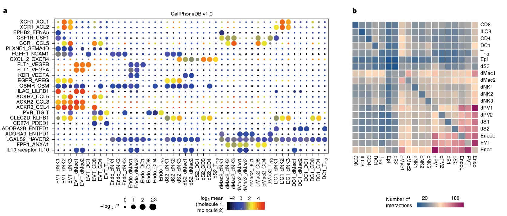
9. Efremova, M., Vento-Tormo, M., Teichmann, S.A. & Vento-Tormo, R. (2020). CellPhoneDB: inferring cell-cell communication from combined expression of multi-subunit ligand-receptor complexes. Nature Protocols, 15(4), 1484–1506. DOI: 10.1038/s41596-020-0292-x

10. Tang, F., Barbacioru, C., Wang, Y. et al. (2009). mRNA-Seq whole-transcriptome analysis of a single cell. Nature Methods, 6(5), 377–382. DOI: 10.1038/nmeth.1315

11. Zheng, G.X.Y., Terry, J.M., Belgrader, P. et al. (2017). Massively parallel digital transcriptional profiling of single cells. Nature Communications, 8, 14049. DOI: 10.1038/ncomms14049

12. Svensson, V., Vento-Tormo, R. & Teichmann, S.A. (2018). Exponential scaling of single-cell RNA-seq in the past decade. Nature Protocols, 13(4), 599–604. DOI: 10.1038/nprot.2017.149

13. Hao, Y., Stuart, T., Kowalski, M.H. et al. (2024). Dictionary learning for integrative, multimodal and scalable single-cell analysis. Nature Biotechnology, 42(2), 293–304. DOI: 10.1038/s41587-023-01767-y

14. Wolf, F.A., Angerer, P. & Theis, F.J. (2018). SCANPY: large-scale single-cell gene expression data analysis. Genome Biology, 19, 15. DOI: 10.1186/s13059-017-1382-0

15. Regev, A., Teichmann, S.A., Lander, E.S. et al. (2017). The Human Cell Atlas. eLife, 6, e27041. DOI: 10.7554/eLife.27041

16. The Tabula Sapiens Consortium, Jones, R.C., Karkanias, J. et al. (2022). The Tabula Sapiens: A multiple-organ, single-cell transcriptomic atlas of humans. Science, 376(6594), eabl4896. DOI: 10.1126/science.abl4896

17. Abdulla, S., Aevermann, B., Assis, P. et al. (2025). CZ CELLxGENE Discover: a single-cell data platform for scalable exploration, analysis and modeling of aggregated data. Nucleic Acids Research, 53(D1), D886–D900. DOI: 10.1093/nar/gkae1142

18. Yost, K.E., Satpathy, A.T., Wells, D.K. et al. (2019). Clonal replacement of tumor-specific T cells following PD-1 blockade. Nature Medicine, 25, 1251–1259. DOI: 10.1038/s41591-019-0522-3

19. van den Brink, S.C., Sage, F., Vértesy, Á. et al. (2017). Single-cell sequencing reveals dissociation-induced gene expression in tissue subpopulations. Nature Methods, 14(10), 935–936. DOI: 10.1038/nmeth.4437

20. O’Flanagan, C.H., Campbell, K.R., Zhang, A.W. et al. (2019). Dissociation of solid tumor tissues with cold active protease for single-cell RNA-seq minimizes conserved collagenase-associated stress responses. Genome Biology, 20, 210. DOI: 10.1186/s13059-019-1830-0

21. Adam, M., Potter, A.S. & Potter, S.S. (2017). Psychrophilic proteases dramatically reduce single-cell RNA-seq artifacts: a molecular atlas of kidney development. Development, 144(19), 3625–3632. DOI: 10.1242/dev.151142

22. Denisenko, E., Guo, B.B., Jones, M. et al. (2020). Systematic assessment of tissue dissociation and storage biases in single-cell and single-nucleus RNA-seq workflows. Genome Biology, 21, 130. DOI: 10.1186/s13059-020-02048-6

23. Tosti, L., Hang, Y., Debnath, O. et al. (2021). Single-Nucleus and In Situ RNA-Sequencing Reveal Cell Topographies in the Human Pancreas. Gastroenterology, 160(4), 1330–1344.e11. DOI: 10.1053/j.gastro.2020.11.010

24. Bakken, T.E., Hodge, R.D., Miller, J.A. et al. (2018). Single-nucleus and single-cell transcriptomes compared in matched cortical cell types. PLoS ONE, 13(12), e0209648. DOI: 10.1371/journal.pone.0209648

25. Lun, A.T.L., Riesenfeld, S., Andrews, T. et al. (2019). EmptyDrops: distinguishing cells from empty droplets in droplet-based single-cell RNA sequencing data. Genome Biology, 20, 63. DOI: 10.1186/s13059-019-1662-y

26. Fleming, S.J., Chaffin, M.D., Arduini, A. et al. (2023). Unsupervised removal of systematic background noise from droplet-based single-cell experiments using CellBender. Nature Methods, 20(9), 1323–1335. DOI: 10.1038/s41592-023-01943-7

27. Young, M.D. & Behjati, S. (2020). SoupX removes ambient RNA contamination from droplet-based single-cell RNA sequencing data. GigaScience, 9(12), giaa151. DOI: 10.1093/gigascience/giaa151

28. Yang, S., Corbett, S.E., Bhoj, V. et al. (2020). Decontamination of ambient RNA in single-cell RNA-seq with DecontX. Genome Biology, 21, 57. DOI: 10.1186/s13059-020-1950-6

29. Caskey, M., Rich, J., Weber, R., Mortazavi, A., Pachter, L. & Hallgrimsdottir, I. (2026). Single-Cell Genomics Decontamination with CellSweep. bioRxiv (preprint). DOI: 10.64898/2026.03.04.709349

30. Wolock, S.L., Lopez, R. & Klein, A.M. (2019). Scrublet: Computational Identification of Cell Doublets in Single-Cell Transcriptomic Data. Cell Systems, 8(4), 281–291.e9. DOI: 10.1016/j.cels.2018.11.005

31. Hao, Y., Hao, S., Andersen-Nissen, E. et al. (2021). Integrated analysis of multimodal single-cell data. Cell, 184(13), 3573–3587.e29. DOI: 10.1016/j.cell.2021.04.048

32. Domínguez Conde, C., Xu, C., Jarvis, L.B. et al. (2022). Cross-tissue immune cell analysis reveals tissue-specific features in humans. Science, 376(6594), eabl5197. DOI: 10.1126/science.abl5197

33. Zhang, X., Lan, Y., Xu, J. et al. (2023). CellMarker: a manually curated resource for comprehensively collecting cell markers. Nucleic Acids Research, 51(D1), D1007–D1015. DOI: 10.1093/nar/gkac947

34. Franzén, O., Gan, L.-M. & Björkegren, J.L.M. (2019). PanglaoDB: a web server for exploration of mouse and human single-cell RNA sequencing data. Database, 2019, baz046. DOI: 10.1093/database/baz046

35. Karlsson, M., Zhang, C., Méar, L. et al. (2021). A single-cell type transcriptomics map of human tissues. Science Advances, 7(31), eabh2169. DOI: 10.1126/sciadv.abh2169

36. Ianevski, A., Giri, A.K. & Aittokallio, T. (2022). Fully-automated and ultra-fast cell-type identification using specific marker combinations from single-cell transcriptomic data. Nature Communications, 13, 1246. DOI: 10.1038/s41467-022-28803-w

37. Han, X., Zhou, Z., Fei, L. et al. (2020). Construction of a human cell landscape at single-cell level. Nature, 581, 303–309. DOI: 10.1038/s41586-020-2157-4

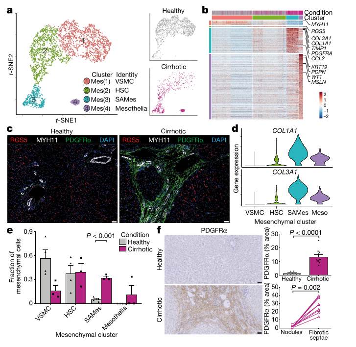
38. Ramachandran, P., Dobie, R., Wilson-Kanamori, J.R. et al. (2019). Resolving the fibrotic niche of human liver cirrhosis at single-cell level. Nature, 575, 512–518. DOI: 10.1038/s41586-019-1631-3

39. Smillie, C.S., Biton, M., Ordovas-Montanes, J. et al. (2019). Intra- and Inter-cellular Rewiring of the Human Colon during Ulcerative Colitis. Cell, 178(3), 714–730.e22. DOI: 10.1016/j.cell.2019.06.029

40. Habermann, A.C., Gutierrez, A.J., Bui, L.T. et al. (2020). Single-cell RNA sequencing reveals profibrotic roles of distinct epithelial and mesenchymal lineages in pulmonary fibrosis. Science Advances, 6(28), eaba1972. DOI: 10.1126/sciadv.aba1972

41. Mathys, H., Davila-Velderrain, J., Peng, Z. et al. (2019). Single-cell transcriptomic analysis of Alzheimer’s disease. Nature, 570, 332–337. DOI: 10.1038/s41586-019-1195-2

42. Liao, M., Liu, Y., Yuan, J. et al. (2020). Single-cell landscape of bronchoalveolar immune cells in patients with COVID-19. Nature Medicine, 26, 842–844. DOI: 10.1038/s41591-020-0901-9

43. Badia-i-Mompel, P., Vélez Santiago, J., Braunger, J. et al. (2022). decoupleR: ensemble of computational methods to infer biological activities from omics data. Bioinformatics Advances, 2(1), vbac016. DOI: 10.1093/bioadv/vbac016

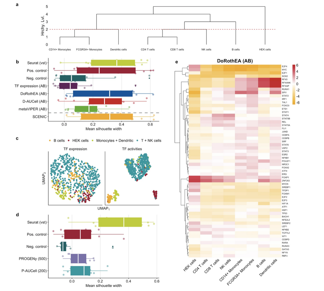
44. Garcia-Alonso, L., Holland, C.H., Ibrahim, M.M. et al. (2019). Benchmark and integration of resources for the estimation of human transcription factor activities. Genome Research, 29(8), 1363–1375. DOI: 10.1101/gr.240663.118

45. Schubert, M., Klinger, B., Klünemann, M. et al. (2018). Perturbation-response genes reveal signaling footprints in cancer gene expression. Nature Communications, 9, 20. DOI: 10.1038/s41467-017-02391-6

46. Holland, C.H., Tanevski, J., Perales-Patón, J. et al. (2020). Robustness and applicability of transcription factor and pathway analysis tools on single-cell RNA-seq data. Genome Biology, 21, 36. DOI: 10.1186/s13059-020-1949-z

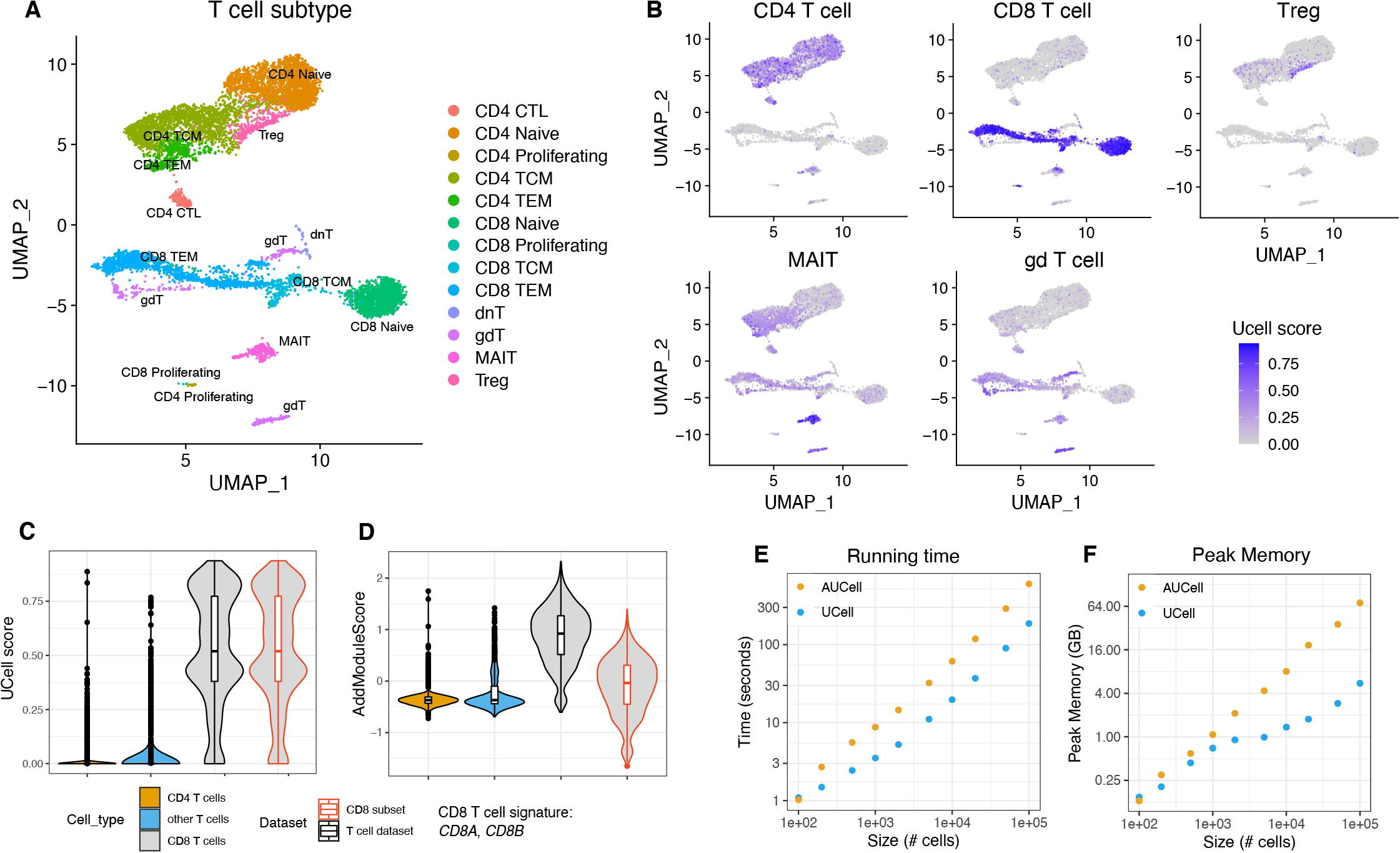
47. Andreatta, M. & Carmona, S.J. (2021). UCell: Robust and scalable single-cell gene signature scoring. Computational and Structural Biotechnology Journal, 19, 3796–3798. DOI: 10.1016/j.csbj.2021.06.043

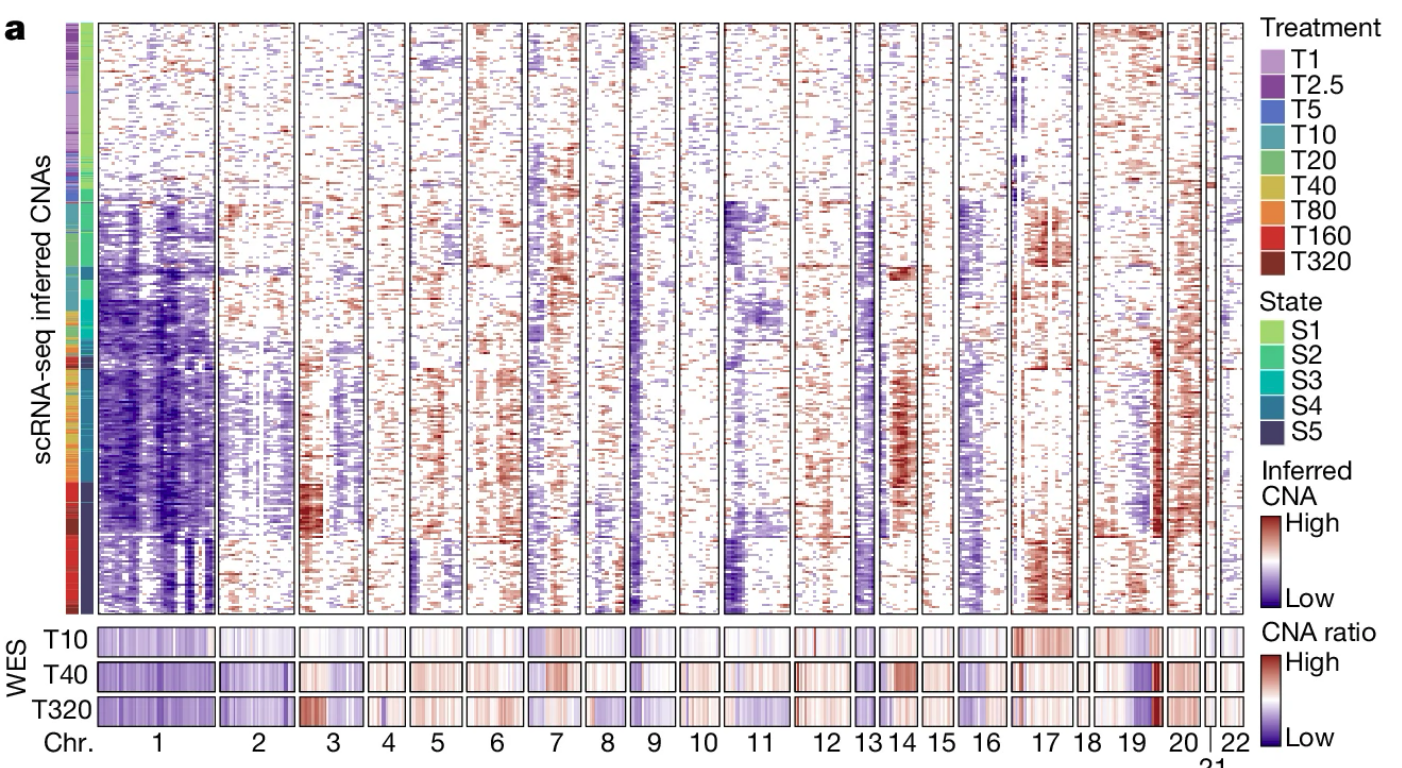
48. Patel, A.P., Tirosh, I., Trombetta, J.J. et al. (2014). Single-cell RNA-seq highlights intratumoral heterogeneity in primary glioblastoma. Science, 344(6190), 1396–1401. DOI: 10.1126/science.1254257. This is the foundational study where the expression-based CNA-inference approach was first introduced and applied to glioblastoma, and on which inferCNV is based; inferCNV itself does not have a dedicated method paper. inferCNV repository: github.com/broadinstitute/infercnv. Recommended actively-maintained alternatives: infercna (github.com/jlaffy/infercna) and CopyKAT (see ref. [49]).

49. Gao, R., Bai, S., Henderson, Y.C. et al. (2021). Delineating copy number and clonal substructure in human tumors from single-cell transcriptomes. Nature Biotechnology, 39, 599–608. DOI: 10.1038/s41587-020-00795-2. CopyKAT repository: github.com/navinlabcode/copykat.

50. De Falco, A., Caruso, F., Su, X.D. et al. (2023). A variational algorithm to detect the clonal copy number substructure of tumors from scRNA-seq data. Nature Communications, 14, 1074. DOI: 10.1038/s41467-023-36790-9

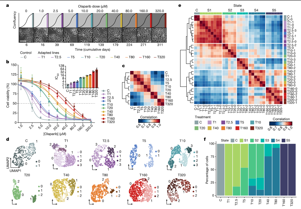
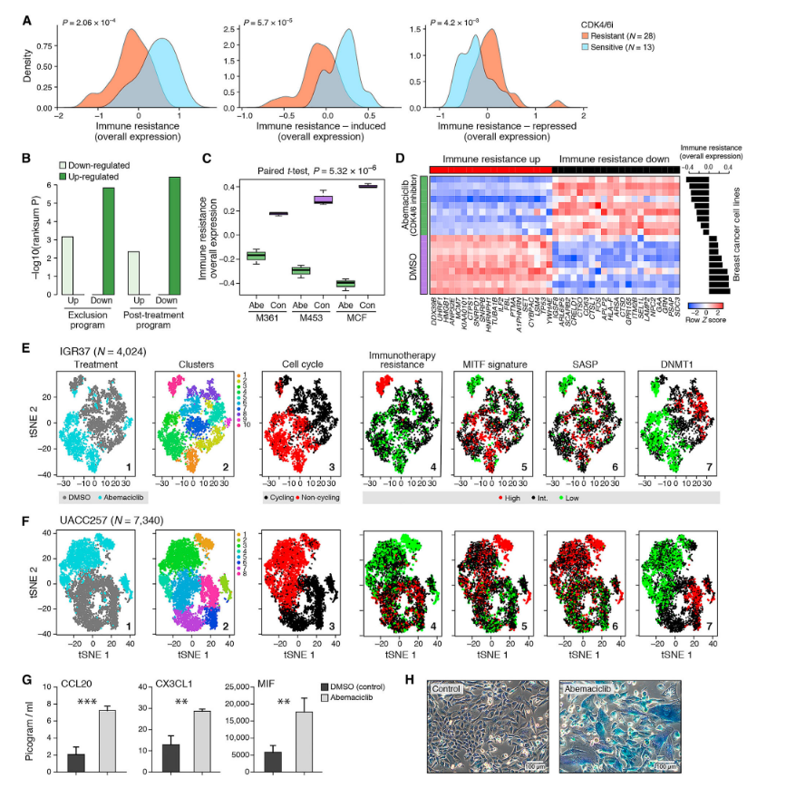
51. França, G.S., Baron, M., King, B.R. et al. (2024). Cellular adaptation to cancer therapy along a resistance continuum. Nature, 631, 876–883. DOI: 10.1038/s41586-024-07690-9

52. Vento-Tormo, R., Efremova, M., Botting, R.A. et al. (2018). Single-cell reconstruction of the early maternal-fetal interface in humans. Nature, 563, 347–353. DOI: 10.1038/s41586-018-0698-6

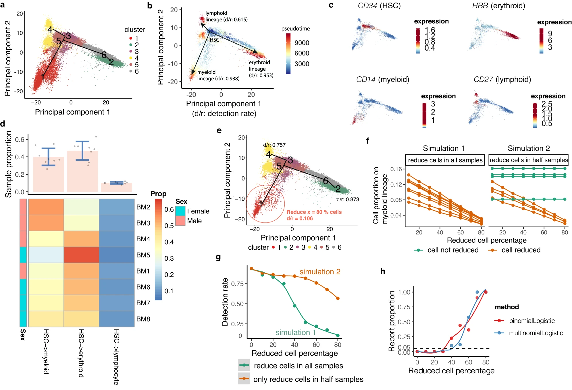
53. Street, K., Risso, D., Fletcher, R.B. et al. (2018). Slingshot: cell lineage and pseudotime inference for single-cell transcriptomics. BMC Genomics, 19, 477. DOI: 10.1186/s12864-018-4772-0

54. La Manno, G., Soldatov, R., Zeisel, A. et al. (2018). RNA velocity of single cells. Nature, 560, 494–498. DOI: 10.1038/s41586-018-0414-6

55. Hou, W., Ji, Z., Chen, Z. et al. (2023). A statistical framework for differential pseudotime analysis with multiple single-cell RNA-seq samples. Nature Communications, 14, 7286. DOI: 10.1038/s41467-023-42841-y

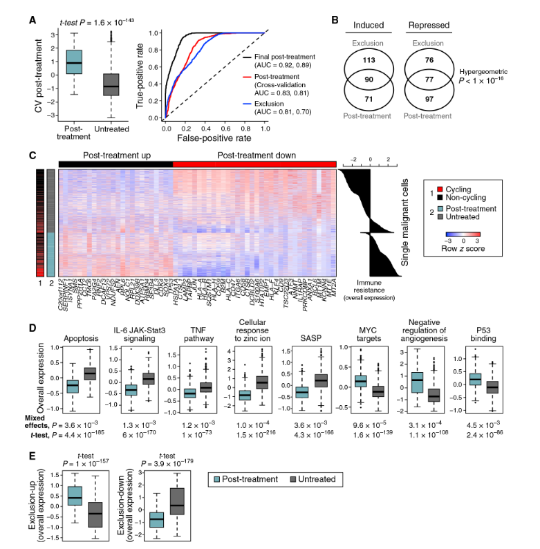
56. Jerby-Arnon, L., Shah, P., Cuoco, M.S. et al. (2018). A Cancer Cell Program Promotes T Cell Exclusion and Resistance to Checkpoint Blockade. Cell, 175(4), 984–997.e24. DOI: 10.1016/j.cell.2018.09.006

57. Martin, J.C., Chang, C., Boschetti, G. et al. (2019). Single-Cell Analysis of Crohn’s Disease Lesions Identifies a Pathogenic Cellular Module Associated with Resistance to Anti-TNF Therapy. Cell, 178(6), 1493–1508.e20. DOI: 10.1016/j.cell.2019.08.008

58. Rambow, F., Rogiers, A., Marin-Bejar, O. et al. (2018). Toward Minimal Residual Disease-Directed Therapy in Melanoma. Cell, 174(4), 843–855.e19. DOI: 10.1016/j.cell.2018.06.025

59. Fustero-Torre, C., Jiménez-Santos, M.J., García-Martín, S., Carretero-Puche, C., García-Jimeno, L., Ivanchuk, V., Di Domenico, T., Gómez-López, G. & Al-Shahrour, F. (2021). Beyondcell: targeting cancer therapeutic heterogeneity in single-cell RNA sequencing data. Genome Medicine, 13, 187. DOI: 10.1186/s13073-021-00978-9

60. He, B., Xiao, Y., Liang, H. et al. (2023). ASGARD is A Single-cell Guided Pipeline to Aid Repurposing of Drugs. Nature Communications, 14, 993. DOI: 10.1038/s41467-023-36637-3

61. Pellecchia, S., Viscido, G., Franchini, M. & Gambardella, G. (2023). Predicting drug response from single-cell expression profiles of tumours. BMC Medicine, 21, 476. DOI: 10.1186/s12916-023-03182-1

62. Gustafsson, J., Held, F., Robinson, J.L. et al. (2024). scDrugPrio: a framework for the analysis of single-cell transcriptomics to address multiple problems in precision medicine in immune-mediated inflammatory diseases. Genome Medicine, 16, 42. DOI: 10.1186/s13073-024-01314-7

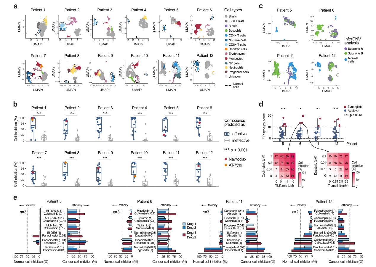
63. Ianevski, A., Nader, K., Driva, K. et al. (2024). Single-cell transcriptomes identify patient-tailored therapies for selective co-inhibition of cancer clones. Nature Communications, 15, 8579. DOI: 10.1038/s41467-024-52980-5

64. Lotfollahi, M., Wolf, F.A. & Theis, F.J. (2019). scGen predicts single-cell perturbation responses. Nature Methods, 16, 715–721. DOI: 10.1038/s41592-019-0494-8

65. Lotfollahi, M., Klimovskaia Susmelj, A., De Donno, C. et al. (2023). Predicting cellular responses to complex perturbations in high-throughput screens. Molecular Systems Biology, 19, e11517. DOI: 10.15252/msb.202211517

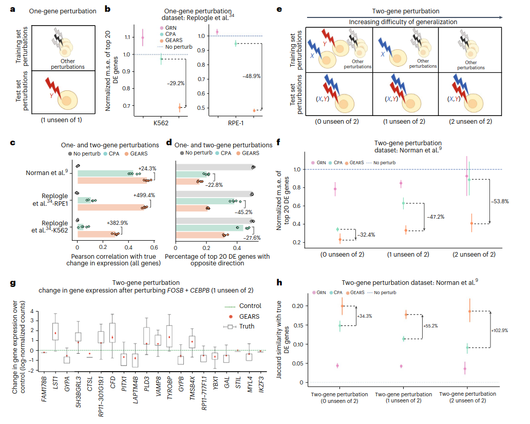
66. Roohani, Y., Huang, K. & Leskovec, J. (2024). Predicting transcriptional outcomes of novel multigene perturbations with GEARS. Nature Biotechnology, 42, 927–935. DOI: 10.1038/s41587-023-01905-6

67. Kernfeld, E.M., Keener, R. & Garmire, L.X. (2025). Deep-learning-based gene perturbation effect prediction does not yet outperform simple linear baselines. Nature Methods. DOI: 10.1038/s41592-025-02772-6

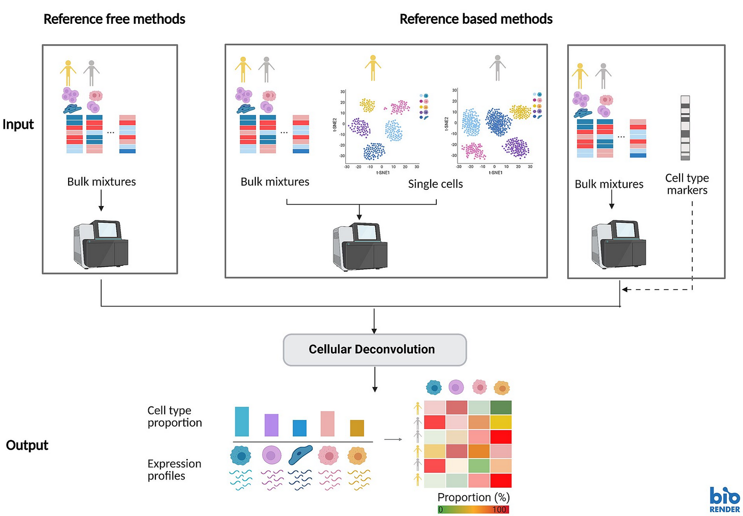
68. Tsoucas, D., Dong, R., Chen, H. et al. (2019). Accurate estimation of cell-type composition from gene expression data. Nature Communications, 10, 2975. DOI: 10.1038/s41467-019-10802-z

69. Chu, T., Wang, Z., Pe’er, D. & Bhatt, P. (2022). Cell type and gene expression deconvolution with BayesPrism enables Bayesian integrative analysis across bulk and single-cell RNA sequencing in oncology. Nature Cancer, 3, 505–517. DOI: 10.1038/s43018-022-00356-3

70. Xu, X., Li, R., Mo, O. et al. (2025). Cell-type deconvolution for bulk RNA-seq data using single-cell reference: a comparative analysis and recommendation guideline. Briefings in Bioinformatics, 26(1), bbaf031. DOI: 10.1093/bib/bbaf031